R E S E A R C H
Open Access
A fuzzy semi-infinite optimization problem
Abd El-Monem A Megahed
**Correspondence:
[email protected] Permanent address: Department of Basic Science, Faculty of Computers and Informatics, Suez Canal University, Ismalia, Egypt Present address: Department of Mathematics, College Of Science, Majmaah University, Al-Zulfi, KSA
Abstract
In this paper, we present a fuzzy semi-infinite optimization problem. Moreover, we will deduce the Fritz-John and Kuhn-Tucker necessary conditions of this problem. Finally, a numerical example is given to illustrate the results.
MSC: 90C34; 90C05; 90C70; 90C30; 90C46
Keywords: fuzzy; semi-infinite; optimization; necessary conditions
1 Introduction
In many practical problems, we might have information containing some uncertainty, which is treated in this paper as fuzzy information; the considered semi-infinite optimiza-tion problem with fuzzy informaoptimiza-tion is a fuzzy semi-infinite optimizaoptimiza-tion problem.
Fuzzy set theory was introduced into conventional linear programming by Zimmer-mann [], fuzzy mathematical programming was presented in [], and fuzzy programming and linear programming with several objective functions were presented by [].
Optimality conditions of a nonlinear programming problem with fuzzy parameters are established, and a fuzzy function is defined, with its differentiability, convexity, and some important properties being studied in []; the fuzzy solution of optimization problems and the incentive solution of the optimization problems are presented which explain that the solution of optimization problems is a generalization of the solutions in the case of crisp optimization problems []. As regards fuzzy mathematical programming: theory, application, and an extension are presented in [].
This paper is organized as follows: In Section , the formulation of the problem of semi-infinite optimization is considered. In Section , the main section of the paper, we will study a fuzzy semi-infinite optimization problem, and the Fritz-John and Kuhn-Tucker necessary conditions. Finally, the conclusion is drawn in Section .
2 A semi-infinite programming problem
A semi-infinite programming problem is an optimization problem in which finitely many variables appear with infinitely many constraints [, ], and we consider a generalized semi-infinite optimization problem (GSIP) [, ] of the form
min
x f(x) s.t.x∈M,
M=
x∈Rn/h
i(x) = ,i∈I,G(x,y)≥
for ally∈Y(x)
,
whereY(x) =y∈Rr/u
k(x,y) = ,k∈K,vl(x,y)≥,l∈L
.
⎫ ⎪ ⎪ ⎪ ⎪ ⎬ ⎪ ⎪ ⎪ ⎪ ⎭
(.)
I,K, andLare finite index sets with|l|<nand|K|<r(where|·|denotes the cardinality), all appearing functions are real valued and continuously differentiable, and the setY(x) is compact for eachx∈Rn, and the set-valued mappingY:x∈Rn→Y(x)⊂Rnis upper semi-continuous at eachx∈Rn.
For the special case that the setY(x) =Y does not depend on the variablex, this prob-lem is a common semi-infinite probprob-lem (SIP). The generalized semi-infinite and bi-level optimization problem are presented by Stein and Still []. Bi-level problems are of the following form.
(BL):
min
x f(x) s.t.x∈Mandyis a solution of (.)
min
y G(x,y)
s.t.y∈Y(x).
The generalized semi-infinite programming on generic local minimizers was introduced by Gunzelet al.[]. The feasible set in generalized semi-infinite optimization is presented by Jongenet al.in []. Furthermore, the linear and linearized generalized semi-infinite optimization problems were introduced by Rukmann []. In [], a first-order optimal-ity condition in generalized semi-infinite programming is introduced. Still discussed the optimality conditions for generalized semi-infinite programming problems in [].
3 A fuzzy semi-infinite programming problem
3.1 Problem formulation
A fuzzy semi-infinite programming problem is defined as
min
x f(x) s.t.x∈M,
whereM=
x∈Rn/hi(x) = ,i∈I,G(x,y)≥
for ally∈Y(x)
,
Y(x) =y∈Rr/u
k(x,y) = ,k∈K,vl(x,y)≥,l∈L
.
⎫ ⎪ ⎪ ⎪ ⎪ ⎬ ⎪ ⎪ ⎪ ⎪ ⎭
(.)
All functions of this problem have the same properties as the problem (.). Forx∈M denote the index sets of the active inequality constraints by
Y(x) =
y∈Y(x)/G(x,y) = , (.)
L(x,y) =
l∈L/vl(x,y) = fory∈Y(x)
.
3.2 Lower level problem
Consider the following lower level problem:
min
y G(x,y)
s.t.y∈Y(x). ⎫ ⎬
⎭ (.)
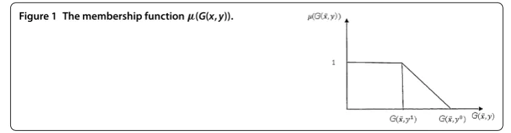
Figure 1 The membership functionμ(G(x,y)).
G(x,y) <G(x,y) <G(x,y), whereμ(G(x,y)) is defined by
μG(x,y)= ⎧ ⎪ ⎨ ⎪ ⎩
, G(x,y)≤G(x,y), G(x,y)–G(x,y)
G(x,y)–G(x,y), G(x,y)≤G(x,y)≤G(x,y), , G(x,y)≥G(x,y),
(.)
whereG(x,y) andG(x,y) denote the values of the objective function of the lower level
problem (.) with the degree of the membership function and , respectively, i.e., G(x,y) is an undesirable value andG(x,y) is a desirable value of the objective function
G(x,y).
Definition The α-level set of the fuzzy goal G(x,y) is defined as the ordinary set Lα(G(x,y)); for the value ofG(x,y) the degree of its membership function exceeds the levelα,i.e.
LαG(x,y)=G(x,y)/μG(x,y)≥α,α∈(, ),
where α is the least acceptable degree of the required value. For certain degreesα the problem (.) can be transformed into the following equivalent form:
min
y G(x,y)
s.t.y∈Y(x),
μ(G(x,y))≥α. ⎫ ⎪ ⎪ ⎬ ⎪ ⎪
⎭ (.)
Ifx∈Mandy∈Y(x), thenyis a minimizer of the problem (.).
By the Fritz-John conditions there exist coefficients λ,β = (βk,k∈ K), γ = (γl,l ∈ L(x,y)), andνsatisfying
DyL(x,y)(x,y,λ,β,γ,ν) = and λ+ν+
k∈K
|βk|+
l∈L(x,y)
γl= , (.)
λ≥,γl≥,ν≥,l∈L(x,y),
where
L(x,y)(x,y,λ,β,γ,ν) =λG(x,y) –vμG(x,y)–α– k∈K
βiuk(x,y) –
l∈L(x,y)
γlvl.
In other words, forx∈Mandy∈Y(x) the setF(x,y) ={(λ,β,γ,v)∈R×R|k|×R|L(x,y)|×
4 Fritz-John conditions
Firstly, we will give some lemmas, definitions, and a proposition which will be used in the proof of the Fritz-John conditions.
Lemma [] Let xt∈M,yt∈Y(xt)and xt→x.Then the set{yt,t∈N}is bounded,and
y∈Y(x)whenever yt→y.
Lemma [] Let l=φ,and for x∈M let Y(x) =φ.Then x is an interior point of M.
Definition Forx∈Mdefine
V(x) =
y∈Y(x)
DxL(x,y)(x,y,λ,β,γ,ν)/(α,β,γ)∈F(x,y)
. (.)
Lemma [] Let x∈M.Then the set V(x)is compact.
Definition [] For a setV, we defineConv(V) to denote the convex hull ofV,i.e. x∈Conv(V) if and only if
x=
n
i=
λixi, xi∈V, n
i=
λi= ,λi≥, (.)
i.e.Conv(V) consists of all finite convex combinations of the elements ofV.
Lemma [] Let V⊂Rnbe a nonempty compact set.Then there exists aξ ∈Rnwith
sTξ> for all s∈V if and only if /∈Conv(V).
Lemma [] Let I,I be finite index sets and si∈Rn,i∈I,and zj∈Rn, j∈I.Then
either(i)or(ii)holds.
(i) There are real numbersai,i∈I,bj≥,j∈I,satisfying
i∈I
aisi+
j∈I
bjzj= ,
i∈I |ai|+
j∈I bj= .
(.)
(ii) The set{si,i∈I}is linearly independent and there exists aξ∈Rnwith
siTξ= , i∈I,
zjTξ> , j∈I. (.) Proposition [] For t∈R and y∈Rr,we define the following functions:
uk(t,y) =uk(x+tξ,y), k∈K,
vl(t,y) =vl(x+tξ,y), l∈L,
G(t,y) =G(x+tξ,y).
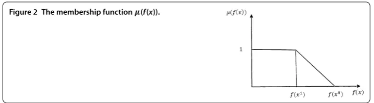
Figure 2 The membership functionμ(f(x)).
(i) The set{Duk(,y),k∈K}(={[Dxuk(x,y)ξ,Dyuk(x,y)],k∈K})is linearly independent.
(ii) There is aw∈Rr+satisfying
DG(,y)w> , Duk(,y)w= ,k∈K,
Dvk(,y)w< ,l∈L(Ex,y).
⎫ ⎪ ⎬ ⎪
⎭ (.)
The fuzzy requirements of the problem (.) can be quantified by electing a membership functionμ(f(x)) (Figure ) which is differentiable in the open intervalf(x) <f(x) <f(x)
whereμ(f(x)) is defined by
μf(x)= ⎧ ⎪ ⎨ ⎪ ⎩
, f(x)≤f(x), f(x)–f(x)
f(x)–f(x), f(x
)≤f(x)≤f(x),
, f(x)≥f(x),
(.)
wheref(x) andf(x) denote the values of the objective function of the problem (.) with the degree of membership function and , respectively,i.e.,f(x) is an undesirable value
andf(x) is a desirable value of the objective functionf(x). For a certain degreeα the
defuzzification of the problem (.) is
min
x f(x) s.t.x∈M,
whereM=
x∈Rn/h
i(x) = ,i= , . . . ,m,G(x,y)≥
for ally∈Y(x)
,
Y(x) =y∈Rr/uk(x,y) = ,k∈K,vl(x,y)≥,l∈L
,
μf(x)≥α, α∈(, ),
μG(x,y)≥α, α∈(, ).
(.)
Theorem Let x be a local minimizer of the problem(.).Then either Y(x)=φand
there exist
yj∈Y
(x),j= , . . . ,p,
(λj,βj,γj,vj)∈F(x,yj),j= , . . . ,p, k≥,η≥,ρi,i∈I,ζj≥,j= , . . . ,p,
⎫ ⎪ ⎬ ⎪
satisfying
k+η+i∈I|ρi|+
p j=ζj>
as well as kDf(x) –ηD(μ(f(x) –α)) –
i∈IρiDhi(x)
–pj=ζjDxL(x,y j)
(x,yj,λj,βj,γj,νj) = , ⎫ ⎪ ⎪ ⎪ ⎬ ⎪ ⎪ ⎪ ⎭
(.)
or Y(x) =φand there exist k≥,η≥,ρi,i∈I,satisfying
k+η+i∈I|ρi|> ,
kDf(x) –ηD(μ(f(x) –α)) –i∈IρiDhi(x) = .
(.)
Proof Letxbe a local minimizer of the problem (.). We distinguish three cases. Case : The set{Dhi(x),i∈I}is linearly dependent. Then we are done by choosingk= ,
η= ,ζ= in (.) (ifY(x)=φ), ork= ,η= in (.) (ifY(x) =φ) as well as a linear
combinationi∈IρiDhi(x) = with
i∈I|ρi|> .
Case : There exists ay∈Y(x) and the set{Duk(x,y) = ,k∈K}is linearly dependent.
Then there exists a linear combinationk∈KβkDuk(x,y) = ,
k∈K|βk|= and therefore
we havek∈KβkDyuk(x,y) = , (,β, , )∈F(x,y) (withβ= (βk,k∈K)), and
DxL(x,y)(x,y, , ,β, ) =
k∈K
βkDuk(x,y) = . (.)
Case : Neither Case nor Case holds. Then the proof is similar to Theorem . in
[].
5 A constraint qualification
Definition The Mangasarian-Fromovitz constraint qualification (MFCQ) of the
prob-lem (.) is said to hold atxif:
() the set{Dhi(x),i∈I}is linearly independent and () there exists a∈Rnsuch that
for alli∈I:Dhi(x)= , for ally∈Y(x) :DxL(x,y)(x,y,λ,β,γ,ν)> , for all(λ,β,γ,v)∈F(x,y). ⎫ ⎪ ⎬ ⎪
⎭ (.)
Theorem Let x be a local minimizer of the problem(.)and(MFCQ)be satisfied.
Then either Y(x)=φand there exist
yj∈Y
(x),j= , . . . ,p,
(λj,βj,γj,vj)∈F(x,yj),j= , . . . ,p,
k≥,η≥,ρi,i∈I,ζj≥,j= , . . . ,p,
⎫ ⎪ ⎬ ⎪
⎭ (.)
satisfying
k+η+i∈I|ρi|+
p j=ζj>
as well as kDf(x) –ηD(μ(f(x) –α)) –
i∈IρiDhi(x)
–pj=ζjDxL(x,y j)
(x,yj,λj,βj,γj,νj) = , ⎫ ⎪ ⎪ ⎪ ⎬ ⎪ ⎪ ⎪ ⎭
or Y(x) =φand there exist k≥,η≥,ρi,i∈I,satisfying the set
k+η+i∈I|ρi|> ,
kDf(x) –ηD(μ(f(x) –α)) –
i∈IρiDhi(x) = .
(.)
The proof is similar to the proof of Theorem if we choosek= .
Example
minf(x) =
x–
+x,
subject toG(x,y) =y+x,
V(x,y) =x–y.
The lower level problem is
minG(x,y) =y+x,
subject toV(x,y) =x–y.
The optimal solution of the crisp problem is (x,x) = (, ),y= , and (λ,γ) = (, ); and
f(
, ) = ,G(x,y) = .
Let f(x) = and G(x,y) = be undesirable values of the problem, the membership
functions off andGare defined by
μ(f) = f–f
f–f= –
x–
+x–
,
μ(G) = G–G
G–G = –y–x.
The new problem is
minf(x) =
x–
+x,
subject toG(x,y) =y+x,
V(x,y) =x–y,
–
x–
+x–
≥α, α∈(, ),
–y–x≥α, α∈(, ).
The lower level problem is
minG(x,y) =y+x,
V(x,y) =x–y,
then
L(x,y,α,γ,γ) =λ(y+x) –γ
x–y
–γ(–y–x+ –α),
DyL(x,y,α,γ,γ) =λ+ yγ+γ= , theny= –
λ+γ
γ
,λ+γ+γ= .
Since
kDf(x) –γD
μf(x) –α
–βDxL(x,y,λ,γ,γ) = ,
we have
k
x–
+ γ
x–
+βγ= , x=
–
βγ
k+ γ
,
kx+ γx–β(λ+γ) = , x=
β(λ+γ)
k+ γ
;
the solution is ⎧ ⎪ ⎪ ⎪ ⎨ ⎪ ⎪ ⎪ ⎩ ⎡ ⎢ ⎢ ⎢ ⎣
β= .,k= .,γ= .,λ= .,
γ= .,γ= .,
α= .,α= .,x= .,
x= .,y= –.
⎤ ⎥ ⎥ ⎥
⎦,f = .,G= . ⎫ ⎪ ⎪ ⎪ ⎬ ⎪ ⎪ ⎪ ⎭ . 6 Conclusion
In this work, we discussed a fuzzy semi-infinite optimization problem, by considering that the minimum of the objective function is fuzzy (min). The Fritz-John conditions and the constraint qualification are discussed for this problem. Finally, an illustrative example is given to clarify the results.
Competing interests
The author declares that they have no competing interests.
Acknowledgements
The author wants to express his deep thanks and his respect to his faculty, colleagues, the Journal, and Prof. Dr. Rachel M Bernales of the Journal of Editorial office. Also the author wants to express his thanks and respect to Jane Doe who provided medical writing services on behalf of XYZ pharmaceuticals Ltd.
Received: 11 July 2014 Accepted: 5 November 2014 Published:19 Nov 2014
References
1. Zimmermann, H-J: Description and optimization of fuzzy systems. Int. J. Gen. Syst.2, 209-215 (1976) 2. Zimmermann, H-J: Fuzzy mathematical programming. Comput. Oper. Res.10, 291-298 (1983)
3. Zimmermann, H-J: Fuzzy programming and linear programming with several objective functions. Fuzzy Sets Syst.1, 45-55 (1978)
4. Cantão, LAP, Yamakami, A: Nonlinear programming with fuzzy parameters: theory and applications. In: Mohammedian, M (ed.) Proceedings of CIMCA 2003. ISBN:1740880684
5. Jameed, AF, Sadeghi, A: Solving nonlinear programming problem in fuzzy environment. Int. J. Contemp. Math. Sci.
7(4), 159-170 (2012)
6. Luhandjula, MK: Fuzzy mathematical programming: theory, applications and extension. J. Uncertain Syst.1(2), 124-136 (2007)
7. Reemsten, R, Ruckmann, J-J (eds.): Semi-Infinite Programming. Kluwer Academic, Boston (1998)
8. Hettich, R, Kortank, KO: Semi-infinite programming: theory methods, and applications. SIAM Rev.35, 380-429 (1993) 9. Jongen, HT, Ruckmann, J-J, Stein, O: Generalized semi-infinite optimization: a first order optimality condition and
examples. Math. Program.83, 145-158 (1998)
11. Stein, O, Still, G: On generalized semi-infinite optimization and bi-level optimization. Eur. J. Oper. Res.142, 444-462 (2002)
12. Gunzel, H, Jongen, HT, Stein, O: Generalized semi-infinite programming: on generic local minimizers. J. Glob. Optim.
42(3), 413-421 (2008)
13. Jongen, HT, Twilt, F, Weber, G-W: Semi infinite optimization: structure and feasibility of the feasible set. J. Optim. Theory Appl.72, 529-552 (1992)
14. Rukmann, JJ: On linear and liberalized generalized semi-infinite optimization problem. Ann. Oper. Res.101, 191-208 (2001)
15. Ruckmann, J-J, Shapiro, A: First-order optimality conditions in generalized semi-infinite programming. J. Optim. Theory Appl.101, 677-691 (1999)
16. Stein, O, Still, G: On optimality conditions for generalized semi- infinite programming problems. J. Optim. Theory Appl.104, 443-458 (2000)
17. Bazaraa, MS, Shetty, CM: Nonlinear Programming Theory and Algorithms. Wiley, New York (1979) 18. Cheney, EW: Introduction to Approximation Theory. McGraw-Hill, New York (1966)
19. Jongen, HT, Jonker, P, Twilt, F: Nonlinear Optimization inRn. II. Transversality, Flows, Parametric Aspects. Peter Lang,
Frankfurt am Main (1986)
10.1186/1029-242X-2014-457