Improved Time Synchronization Algorithms Based on TPSN

14th International Conference on Wireless Communications, Networking and Mobile Computing (WiCOM 2018) ISBN: 978-1-60595-578-0

Improved Time Synchronization Algorithms Based on TPSN

Xiangli Jia1, Yang Lu12,*, Xing Wei1,2 and Wenjing Tao1

ABSTRACT

When number of levels increases, local clock offset difference also increases for Timing-Sync Protocol for Sensor Networks (TPSN). To address the problem, an algorithm of Timing-Sync Protocol for Sensor Networks of Chain (C-TPSN) is proposed in this paper. It can provide synchronization among the cluster roots first then the cluster roots can synchronize asynchronously with their cluster members hierarchically by dividing the network into a number of clusters, which decreases the cumulative difference and improves the accuracy; Moreover, because the TPSN algorithm, a time deviation synchronization algorithm, needs to perform periodically time synchronization so that message overheads are large. An algorithm of Adaptive Interval Synchronization (Adap-I) is provided to optimize for message overheads on the premise of meeting the requirements of some precision. Finally, NS2 simulation platform is used to simulate and test the algorithms from the aspects of synchronization difference and message overheads. The results show that the C-TPSN algorithm can synchronize more effectively with higher precision, and the Adap-I can optimize for message overheads on the premise of meeting the synchronization accuracy.

Keywords: Wireless Sensor Networks (WSN), Timing-Sync Protocol for Sensor Networks (TPSN), time synchronization, clustering, NS2.

1. INTRODUCTION

The time synchronization technology is a supporting technology for Wireless Sensor Networks (WSN) [1]. Applications such as data fusion, positioning and sleep scheduling in WSN require that the node's clock to be synchronized. Due to the difference of the crystal oscillator and the influence of the external environment, the local clock of each node will be offset. Therefore, there will possibly cause application errors eventually because the input data is incorrectly time stamped and they will not be interpreted correctly by the application. For the time critical applications running on WSN, the clock drift problem should be reduced to a reasonable level or completely eliminated if possible [2].

Due to the limitation characteristic of sensor node energy, computing power, communication bandwidth, and storage capacity [3], the time synchronization algorithm designed is not easy to be too complex. Many scholars have proposed various time synchronization algorithms, among which Timing-Sync Protocol for Sensor Networks (TPSN) [4] is easy to implement and an effective time synchronization algorithm but it has some weaknesses. When number of levels

1

School of Computer Science and Information Engineering, Hefei University of Technology, Hefei Anhui 230601, China

2

Engineering Research Center of Safety Critical Industry Measure and Control Technology, Ministry of Education, Hefei Anhui 230601, China

increases, local clock offset difference also increases. In this paper, two improvements are made to the TPSN algorithm. The first algorithm is the Timing-Sync Protocol for Sensor Networks of Chain (C-TPSN), TPSN can therefore provide synchronization among the cluster roots first then the cluster roots can synchronize asynchronously with their cluster members hierarchically providing different levels of synchronization by dividing the WSN into a number of clusters, which reduces the cumulative difference and thus improves the synchronization accuracy; the second algorithm is the Adaptive Interval Synchronization (Adpt-I), because TPSN algorithm, time deviation synchronization algorithm, needs to perform periodically time synchronization so that message overheads are large. This improvement is designed to optimize for message overheads on the premise of meeting the synchronization accuracy.

Section 2 provides the relevant algorithms of time synchronization and the TPSN algorithm is highlighted, Section 3 details the enhancement algorithms to the TPSN, Section 4 simulates the algorithms by NS2 and draws conclusions and finally the summary is given in Section 5.

2. RELATED WORK

2.1 Clock Model

The purpose of time synchronization research is to make the nodes of a distributed system aware and consistent with time. In order to maintain the reliability and continuity of the local clocks, a time synchronization algorithm does not directly adjust the local hardware clock. Instead, the local time of the sensor node is calibrated by adjusting the logic clock which is actually a function that converts the hardware clock into real time.

The different of sensor nodes crystal frequency then causes a clock drift. It is generally considered that the crystal frequency is constant for a long time, which means the clock drift of the node is constant during a period of time. Hence, the node's logic clock can be expressed by (1) [5].

C t( )_i α t β_i  _i （1）

Where C(t)i is the logical clock of the node i at time t, αi is the clock drift and βi is

the initial time offset of the node i.

2.2 Time Synchronization Algorithms

At present, domestic and foreign researchers have proposed many different time synchronization algorithms due to varying requirements. There are three basic algorithms for the time synchronization in WSN [6]:

1）Sender-Receiver Based Synchronization Mechanism 2）Receiver-Receiver Based Synchronization Mechanism 3）Delay Measurement Based Synchronization Mechanism

time of the packet, and then exchange packets to achieve time synchronization between the nodes. It excludes the influence of the sender on the synchronization accuracy, but the calculation amount and the synchronization overheads are large.

Critical Path Sender S

Receiver A

Receiver B

Figure 1. The principle of the RBS algorithm.

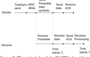
The Delay Measurement Time Synchronization (DMTS) [8] is a kind algorithm of based on one-way message exchange as well as the Delay Measurement mechanism. The basic principle is shown in Figure 2. The master node broadcasts the synchronization message carrying the local sending time, all the receiver nodes measure the time delay and set their time as received master time plus measured time transfer delay to achieve synchronization with the master node. This algorithm does not consider the influence of propagation delay and the clock drift so that the synchronization accuracy is not high.

Sender

Receive

TimeSync. send

MAC delay

Send Preamble Start symbols

Receive Preamble

Send data

Receive data

Receive ACK

Send ACK

Receiver Processing

Time stamp T1

Time stamp T2

Figure 2. The principle of the DMTS algorithm.

The TPSN proposed by Saurabh Ganeriwal et al., two-way message exchange used, is a Sender-Receiver mechanism based time synchronization algorithm for WSN. The basic principle is detailed in section 2.3. The algorithm works in two steps. In the first step, a hierarchical structure is established in the network and then the two-way message exchange is performed along the edges of this structure to establish a global timescale throughout the network. Eventually all nodes in the network synchronize their clocks to a reference node. The synchronization effect of the TPSN is better, while when number of levels increases, local clock offset difference also increases [2, 9]. For this reason we provide significant improvements to the TPSN.

2.3 TPSN

TPSN has two main steps to synchronize a network as Level Discovery Phase and Synchronization Phase [10].

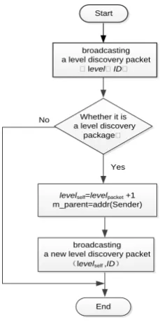
This phase of the algorithm occurs at the onset, when the network is deployed. First a root node is selected and assigned the level 0. The root node initiates this phase. Specifically, the root node broadcasts a level discovery packet, which contains the identity (ID) and the level (0) of the sender. Each node that receives this packet sets its own level as one greater than the level of the received packet. The nodes that a level is set will neglect any such future packets. To avoid collisions, they wait for a random period of time and broadcast a new level discovery packet containing their own level. This process is continued and eventually every node in the network is assigned a level [11]. In short, when a node receives a level discovery packet, it sets its own level as one greater than the level of the received the level discovery packet and sets the sender as its own parent. The node ignores the future level discovery packets if it has been assigned a level. The flow chart of this phase is shown in Figure 3.

Start

Whether it is a level discovery

package？

levelself=levelpacket +1

m_parent=addr(Sender)

broadcasting a new level discovery packet

（levelself ,ID）

End Yes No

broadcasting a level discovery packet

？level？ID？

Figure 3. The flow chart of level discovery phase.

B. Synchronization Phase

The root node broadcasts a time sync packet to initiate Synchronization Phase. When all the one hop neighbors which level is 1 receive this packet, they will perform a two-way message exchange with the root node. However, before performing the two-way message exchange, each node waits for some random time to avoid collisions. In other words, the node in level 1 sends a synchronization pulse packet to the root node (its parent) periodically to request synchronization, the parent node will reply an acknowledgement packet, and once the nodes have receive the packets, they will adjust their clocks to synchronize with the root node. The nodes in level 2 will listen to this process and perform the two-way message exchange with their parent nodes which level is 1 after waiting for some random time. This randomness is to allow nodes in level 1 to complete synchronization with the root node. This process is done until all nodes in the network have synchronized to the root node [12].

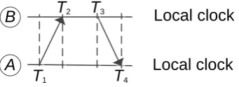
the ‘A’ synchronizes to the ‘B’, T1, T4 represent the time measured by the local clock

of ‘A’. Similarly, T2, T3 represent the time measured by the local clock of ‘B’. 4

timestamps are obtained from the MAC layer.

T4

T2

T1

T3

A

B Local clock

Local clock

Figure 4. Two-way message exchange between pair of nodes.

Step 1 At time T1, ‘A’ sends a synchronization pulse packet to ‘B’. The

synchronization pulse packet contains the level number of ‘A’ and T1.

Step 2 ‘B’ receives this packet at time T2, where T2 is equal to T1 + δ + d. Here δ

and d represents the clock drift between the two nodes and propagation delay respectively, assuming that the clock drift and the propagation delay do not change in this small span of time.

Step 3 At time T3, ‘B’ sends back an acknowledgement packet to ‘A’. The

acknowledgement packet contains the level number of ‘B’ and T1, T2 and T3.

Step 4 ‘A’ receives the packet at time T4.

Step 5 Finally, ‘A’ can calculate the clock drift and propagation delay by (2) and (3) and corrects its own time to complete the synchronization [13].

δ （T2T1）-₂（T4T3） (2)

d （T2T）（1₂ T 4T） ₍₃₎ 3

3. ENHANCEMENT ALGORITHMS TO TPSN

3.1 C-TPSN

A. Cluster network structure establishment

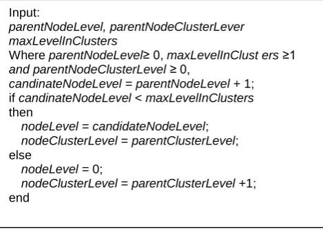
This algorithm improves directly the Level Discovery Phase of TPSN. There is a directed spanning tree that the TPSN algorithm generates. In order to divide a network into clusters, the level parameter in TPSN is used and a similar level parameter is introduced for clusters. So each node will have a level and a cluster (or group) level. The nodes in the same cluster have the same cluster level and the cluster level of the next cluster is larger than that of the upper cluster. A spanning tree is clustered by using the level depth. The level depth equals maxLevelInClusters. When the node's level is greater than maxLevelInClusters, nodes will be in the next cluster and the cluster level is increased by one but the level of nodes is reset to 0 again, the nodes belonging to the level 0 are set as the cluster roots. Otherwise, the cluster level does not change but the level of the node is the parent node's level plus one. Figure 5 shows how a network spanning tree is divided clusters.

Figure 5. Algorithm to form clusters.

If the message complexity of this clustering algorithm is considered as the number of messages exchange between nodes until a valid clustering structure is achieved, it has the same complexity to build a spanning tree, because the network structure was established by broadcasting level discovery packets at level discovery phase. The improved algorithm adds to only the cluster level field and no message exchanges have been added. If n is the number of nodes in the network, a node may receive the number of packets sent from other n-1 nodes so the message complexity is O(n2).

B. Synchronization Phase

When a source node needs to synchronize to a destination node that usually is cluster root, it sends a synchronization pulse packet to its parent node leaf. That leaf transfers the request to its parent and others also do this until the message reaches the destination node. The destination node then replies the time information back using the same path to the request node. For the request node and the destination node, there is no change in the TPSN behavior. For intermediate nodes, the time information of sender needs to be modified. This synchronization method can be done for any node, but since the intermediate nodes which need to continuously participate in the synchronization process, not only the message overheads are large but also the precision might reduce due to they cannot answer synchronization requests when doing another chain synchronization. Therefore, if a cluster member node

Input:

parentNodeLevel,parentNodeClusterLever

maxLevelInClusters

Where parentNodeLevel≥ 0, maxLevelInClust ers ≥1 and parentNodeClusterLevel ≥ 0,

candinateNodeLevel = parentNodeLevel + 1; if candinateNodeLevel < maxLevelInClusters

then

nodeLevel = candidateNodeLevel;

nodeClusterLevel = parentClusterLevel; else

nodeLevel = 0;

synchronizes to the cluster root, the intermediate node on the path is in chain synchronization state and cannot answer other node's synchronization requests then it can reply a reject message to the node just like in TPSN while the child cluster root synchronizes to the parent cluster root whenever possible.

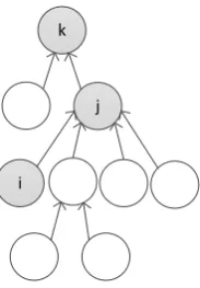
Here is a simple scenario shown in Figure 6 to understand how chain synchronization works. Here i is the source node, requesting synchronization. j is the intermediate node and k is the destination node to be synchronized.

When node i starts the synchronization, it asks for the time to its parent, which is node j. Node j forwards the synchronization request to node k. Before forwarding the request packet, node j needs to store the address and the sent time of requester node i and replace sent time of requester in the packet. When node k receives the forwarded packet, it is just a TPSN packet from node j. So, node k replies the request packet containing its own time to node j. Node j updates its own time when receiving this packet, and then replaces the requester's sent time with the store original sent time in the packet and sends the packet containing its own time information to the node i. With this packet, node i updates its clock correctly.

j

i k

Figure 6. Chain synchronization example.

3.2 Adpt-I

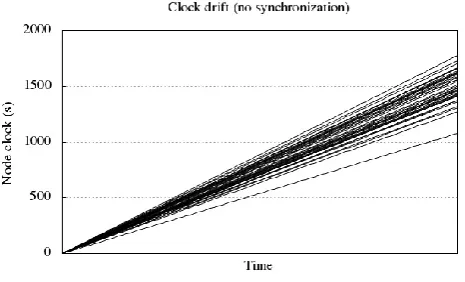
The synchronization difference and message overheads are inextricably linked with the synchronization interval. Decreasing the interval will improve the synchronization but it will also increase the message load on the system. What's more, in most cases, a clock difference up to some value is acceptable. Because the clock drift between nodes is different as seen in Figure 7, the time offset between nodes is different in the same time. So setting the same interval for all nodes is not a reasonable choice. In addition, because of the limited energy of the sensor nodes, it is not reasonable to improve synchronization less for larger message overheads in certain conditions. Therefore, it is a good method that the interval can be adaptive. The purpose of the Adpt-I is to optimize for message overheads while meeting the accuracy.

this paper is 1%. The interval of the nodes can be obtained by (4) and (5). Obviously, if the desired synchronization different is kept small, then it will increase the number of messages. Various desired synchronization different will be selected, and the synchronization interval of the nodes will also be different.

          1 1 1 01 1 1 99 0 b a b a . b a . b a / / / / （4）

i n t e r v a l

*



(

a

/

b

)

Where a is the expected synchronization different, b is the last synchronization result and intevaliis the next synchronization interval of node i.

4. SIMULATION RESULTS ANDANALYSES

4.1 Simulation Environment

In this paper, the NS2 (v2.35) network simulator is used to simulate the TPSN and the improved algorithms respectively. The performance of the algorithms is verified mainly from the synchronization different and the message overheads. The parameters used in the simulation are listed in Table I.

TABLE I. SIMULATION PARAMETERS.

Parameters Values

Network area (m2) 1000*1000

Nodes 40

Simulation duration (s) 1500

Periodic interval (s) 1

Clock drift model N（1,0.001）

A simulation of the WSN with 40 nodes is prepared and all nodes are located in a 1000 m * 1000 m area randomly using uniform distribution. Set the simulation time to 1500 s and the periodic interval to 1 s. Use the normal distribution with parameter μ=1, σ2=0.001 to generate a clock drift of a node, so αi in (1) obeys the N (1, 0.001)

Figure 7. Clock drifts of nodes.

Nodes of WSN are usually randomly arranged. In order to ensure the effectiveness of the algorithms, TPSN, C-TPSN and Adpt-I are simulated respectively by setting diverse seeds to generate different networks. After a large number of simulation experiments, the simulation results of 100 different networks were randomly selected for performance analysis.

The C-TPSN needs to set a level depth to divide a network into clusters. Different a level depth set, the network varies and then the synchronization is also different. When the total levels of network are L, the level depth may be set from 2 to L-1. To study what effect the level depth has on synchronization, the level depth is set from 2 to L-1 when simulate the C-TPSN.

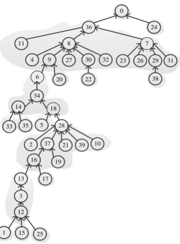
A simple example shows how to generate a cluster network of C-TPSN by setting a level depth. If the seed is assigned 0 and the level depth is set 3, a cluster network topology structure as shown in Figure 8. In this scenario, the total levels of the network are 14 and the nodes in the same horizontal have the same level. In addition, one shadow is a cluster which only has 0-2 three levels and the same cluster has the same cluster level.

0

36 24

11 7

23 8

26 29 31

20

6 ₂₂ 38

34 14

33

3 35

37 _{21 39} 10 2

16 ₁₉

13 17

15 12

1 25

27 32 9 30 4

18

5 28

Figure 8. A cluster network topology of C-TPSN.

4.2 Simulation Results and Analysis

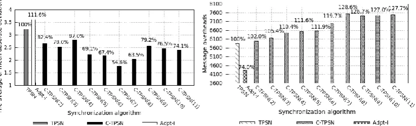
The average value of the network-wide synchronization difference, that is, the average value of the synchronization difference of all nodes in the network with the root node is calculated. The message overheads are the average value of the number of sent and received packets of nodes in the network. Because of the different total levels of the network, the synchronization is not comparable. So analysis is performed on the networks of same total levels. Figure 9 to Figure 15 show the average results of synchronization difference and message overheads when network owns the same total levels. 100 random experiment results of different networks are analyzed. In those figures, C-TPSN (m) indicates that the level depth is set as m when simulate the C-TPSN algorithm, and in the titles, (m) kinds mean the different frequency (m) corresponding to the network of different total levels among the 100 kinds of experimental results extracted.

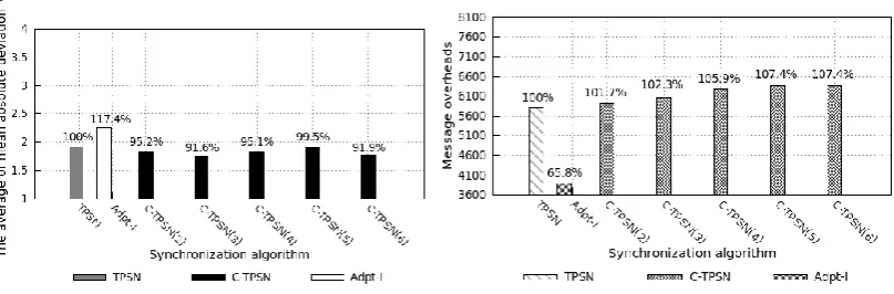
(a) The average of synchronization difference; (b) The average of message overheads Figure 10. Total levels are 7 (17 kinds).

(a) The average of synchronization difference; (b) The average of message overheads Figure 11. Total levels are 8 (20 kinds).

(a) The average of synchronization difference; (b) The average of message overheads Figure 13. Total levels are 10 (17 kinds).

(a) The average of synchronization difference; (b) The average of message overheads Figure 14. Total levels are 11 (7 kinds).

(a) The average of synchronization difference; (b) The average of message overheads Figure 15. Total levels are 12 (4 kinds).

From Figure 9 to Figure 15, it can be seen that no matter how a level depth is set, average synchronization difference of the C-TPSN than the TPSN is smaller, the reduction range is from 54.58% to 99.46%. However, which increases small message overheads that are expected, because the idea of C-TPSN reduces synchronization difference by increasing small message overheads.

message overheads. The level depth which makes increase the smaller message overheads while reduce the more synchronization difference is optimal.

Define the level depth corresponding to the largest one that the weighted difference between reducing the percentage of synchronization difference and increasing the percentage of message overheads is optimal. Where the weight of the reduced synchronization difference percentage is 0.8 and the weight of the increased message overheads percentage is 0.2. It means the cost function z = 0.8x-0.2y, the level depth corresponding to the minimum z value is optimal, where x is the decreased percentage in synchronization difference and y is the increased percentage in message overheads.

Due to the appeared samples of 6 levels, 11 levels and 12 levels are insufficient when 100 different experimental results are sampled. It's hard to derive the regularity. Therefore, only sufficient synchronization samples are considered. The experimental results show that the network has 7 levels, 8 levels, 9 levels and 10 levels respectively, when the level depth is set to 3, 4, 4, and 5 separately, the value of the cost function z is the smallest so the synchronization is the optimum. Therefore, when level depth is set to |L/2|, it may realize comprehensive optimization of synchronization difference and message overheads, where L is the total levels of the network. In other words, the level depth which equals to half integer of the total levels of the network is the best. In this case, the C-TPSN algorithm has the best synchronization result.

When the network has 7 levels, 8 levels, 9 levels and 10 levels respectively, the percentage of synchronization difference that Adpt-I increased is respectively 17.43%, -2.68%, 4.66% and 2.82%, and the reduced percentage of message overheads is successively 34.23%, 31.47%, 29.23% and 30.72%. It can be seen that this algorithm can really reduce the extra message overheads compared to reference TPSN synchronization.

5. CONCLUSION

When number of levels increases, local clock offset difference also increases for TPSN. Considering this problem, this paper proposes the C-TPSN algorithm, which achieves the synchronization between the lower nodes and the cluster roots by dividing a network into clusters. The relationship between the level depth and the total levels of network is studied, which is done to better satisfy a certain need. A large number of experiments have verified that this algorithm can reduce the cumulative error of the whole network. What's more, when level depth is set to |L/2|, it may realize comprehensive optimization of synchronization difference and message overheads Compared with [2], the experiment is more complete and the synchronization is better. This algorithm can be used in places where higher accuracy is demanding. In addition, the Adpt-I algorithm can reduce extra message overheads on the premise of meeting the setting accuracy, which is a good improvement. So there will be extensive applications for energy-constrained WSN.

ACKNOWLEDGMENTS

This work is jointly supported by National Key Research and Development Program (Grant No. 2016YFC0801405, 2016YFC0801804).

REFERENCES

[1] Z. Y. Jiang, Y. Chen, B. Hu, et al. 2017, “Research on time synchronization algorithm for Wireless Sensor Networks,” Computer Engineering and Applications, 53(1):1-8. (in Chinese)

[2] A. B. Kulakli, K. Erciyes. 2008. “Time Synchronization Algorithms based on Timing-Sync Protocol in Wireless Sensor Networks.” 2008 23rd International Symposium on Computer and Information Sciences,pp.1-5.

[3] Jihong Sun, Huanzheng, Shao. 2017, “An Improved Time Synchronization Algorithm for Wireless Sensor Networks” International journal of online engineering. 13(5):67-79 https://doi.org/10.3991/ijoe.v13i05.7049

[4] S. Ganeriwal, R. Kumar, M. B. Srivastava.2003. “Timing-Sync Protocol for Sensor Networks”.

Proceeding of First International conference on Embedded Networked Sensor Systems, pp. 138 - 149.

[5] X. C. Yang. 2016. The Analysis and Research of Improved Time Synchronization Algorithm TPSN for Wireless Sensor Network. Inner Mongolia: Inner Mongolia University. (in Chinese) [6] Y. Jiang, S. X. Guo, J. Q. Gao, et al. 2014. “Low Overhead Time Synchronization Algorithm for

Wireless Sensor Network”. Computer Science, 41(3): 129-131, 158. (in Chinese)

[7] J. Elson, L. Girod, D. Estrin. 2002 “Fine- grained time synchronization using reference broadcasts”. Proceedings of the 5th Symposium on Operation System Design and Implementation, pp. 147 - 163.

[8] P. Su. June 2003. “Delay measurement time synchronization for wireless sensor networks”. Inter Research Center：IR- TR-2003-64.

[9] S. E. Khedir, N. Nasr, A. Kachouri, et al. 2013. “Synchronization in wireless sensors networks using balanced clusters.” 6th Joint IFIP Wireless and Mobile Networking Conference (WMNC.),pp. 1-4.

[10] D. Liu, Z. Y. Zheng, Z. M. Yuan, et al. 2012. “An Improved TPSN Algorithm for Time Synchronization in Wireless Sensor Network.” International Conference on Distributed Computing Systems Workshops, pp. 279-284.

[11] Z. Y. Tao, M. Hu. 2012. “Improvement Based on the Hierarchical Levels Structure of the TPSN Algorithm.” Chinese Journal of Sensors and Actuators, 25(5):691-695. (in Chinese)

[12] S. Rucksana, C. Babu, S. Saranyabharathi. 2015. “Efficient timing-sync protocol in wireless sensor network.” 2015 International Conference on Innovations in Information, Embedded and Communication Systems (ICIIECS), pp. 1–5.

[13] G. Seth, A. Harisha. 2015.“Energy efficient timing-sync Protocol for Sensor Network.” 2015 International Conference on Computing and Network Communications (CoCoNet),pp. 912–916. [14] Benzaid, C. ,Bagaa, M., Younis, M. 2017. “Efficient clock synchronization for clustered wireless