Dai Kou type conjugate gradient methods with a line search only using gradient

R E S E A R C H

Open Access

Dai-Kou type conjugate gradient methods

with a line search only using gradient

Yuanyuan Huang

_{and Changhe Liu}

*_{Correspondence:}

[email protected] School of Mathematics and Statistics, Henan University of Science and Technology, Luoyang, 471023, P.R. China

Abstract

In this paper, the Dai-Kou type conjugate gradient methods are developed to solve the optimality condition of an unconstrained optimization, they only utilize gradient information and have broader application scope. Under suitable conditions, the developed methods are globally convergent. Numerical tests and comparisons with the PRP+ conjugate gradient method only using gradient show that the methods are efficient.

Keywords: conjugate gradient; optimality condition; line search; sufficient descent condition; global convergence

1 Introduction

Consider the following problem of findingx∈Rnsuch that

g(x) = , ()

whereg:Rn_→Rn_{is continuous. Throughout this paper, problem () corresponds to the} first-order optimality condition of the unconstrained optimization

minf(x), ()

wheref :Rn_{→Ris the function whose gradient isg.}

Conjugate gradient methods are very efficient in solving large scale problem (), iff is known, due to their simple iteration and their low memory requirements. For any given starting pointx∈Rn, an iterative sequence{xk}is generated by the following form:

xk+=xk+αkdk, ()

whereαkis a step-length obtained by some line search, anddkis a search direction gen-erated by

dk= ⎧ ⎨ ⎩

–gk, ifk= , –gk+βkdk–, ifk≥,

()

wheregk=g(xk). Different choices of the parameterβkin () lead to different nonlinear conjugate gradient methods. The Fletcher-Reeves [], Hestenes-Stiefel [],

Polyak [, ], Dai-Yuan [] and Liu-Storey [] formulas, and so on, are well-known formu-las forβk. Particularly, conjugate gradient methods with the following (sufficient) descent condition

g_kTdk≤–cgk, ∀k≥,c> , ()

are very important and are always more efficient.

Recently, Dai and Kou [] designed a family of conjugate gradient methods for the un-constrained nonlinear problems, the corresponding search direction is close to the direc-tion of the scaled memoryless BFGS method. More importantly, they satisfied the suf-ficient descent condition (). Numerical experiments illustrated that the Dai-Kou type conjugate gradient methods are more efficient than the Hager-Zhang type methods [] presented by Hager and Zhang [, ]. For other descent conjugate gradient methods pro-posed by researchers, please see [, –] and the references therein.

For conjugate gradient methods, line search plays an important role for the global con-vergence. In general, the weak Wolfe line search,

f(xk+αkdk)≤f(xk) +δαkgkTdk, ()

σg_kTdk≤g(xk+αkdk)Tdk, ()

where  <δ<σ< , was used to obtain the step-lengthαk. Hager and Zhang [] showed that the first condition () may never be satisfied due to the existence of the numerical errors (see also []). Thus, in order to avoid the numerical drawback of the weak Wolfe line search, they proposed approximate Wolfe conditions [, ], which was a combination of the weak Wolfe line search and

σg_kTdk≤g(xk+αkdk)Tdk≤(δ– )gkTdk, ()

where  <δ< / andδ<σ < . Numerical tests showed that the combined line search performed well, but there is no theory to guarantee the global convergence. Then Dai and Kou proposed an improved Wolfe line search, that is, the step-lengthαksatisfied () and

f(xk+αkdk)≤f(xk) +min

g_kTdk,δαkgkTdk+ηk

, ()

where  <δ<σ< ,>  is a constant parameter and{ηk}is a positive sequence satisfying

k≥ηk< +∞. With the improved Wolfe line search, the global convergence of Dai-Kou type conjugate gradient methods was guaranteed.

problem (), the step-lengthαksatisfied

g(xk+αkdk)Tdk+ 

max{–μk, }αkdk _≤σgT

kdk, ()

whereμkis a determined real number and  <σ< . The line search allowed small choices ofαk. In order to avoid this drawback, Dong [] considered the following line search:

σg_kTdk≤g(xk+αkdk)Tdk≤δgkTdk, ()

where  <δ<σ< . Motivated by the work of [], we embed the line search () into the Dai-Kou type conjugate gradient methods, then the improved methods of this paper have several advantages. They have the positive features of the Dai-Kou type methods for problem (), they can be used to solve the nonlinear optimization () only requiring gradient information, and they can be used to solve some systems of nonlinear equations, such as those arising in boundary value problems and others.

The rest of this paper is organized as follows. In the next section, we simply review the Dai-Kou type conjugate gradient methods for unconstrained minimization and de-velop them to solve problem (). In Section , we prove the global convergence of the improved methods under some suitable conditions. In Section , we select two classes of test problems to test the improved methods. One class is composed of test problems from the CUTEst test environment, and the other class is composed of some boundary value problems. The numerical performance is used to confirm their broader application and to compare with that of the PRP+ conjugate gradient method in []. Finally, some conclusions are given in Section .

2 Algorithm

In this section, we describe the details of the proposed methods. First, we briefly review the Dai-Kou type conjugate gradient methods in the setting of unconstrained minimization (). We have mentioned above that nonlinear conjugate gradient methods are identified by the definitions of the parameterβkin (). For the family of Dai-Kou type conjugate gradient methods, the parameterβkis defined as

β_kN(τk–) =max βk(τk–),ηg

T kdk– dk–

. ()

Here,

βk(τk–) = g T kyk–

dT k–yk–

–

τk–+

yk–

sT k–yk–

–s T k–yk– sk–

gT ksk–

dT k–yk–

, ()

whereyk–=gk–gk–,sk–=αk–dk–=xk–xk–,τk–is a parameter corresponding to the scaling parameter in the scaled memoryless BFGS method, andη∈[, ). The parameters

βkin the Dai-Liao type methods [] and the Hager-Zhang type methods [] are special cases of formula (). Ifτk–is specially defined as

withλ∈[, ] and

τ_k–A =yk– 

sT_k–yk–

, ()

τ_k–B =s T k–yk– sk–

, ()

then the Dai-Kou type conjugate gradient methods satisfy the sufficient descent condi-tion ().

The Dai-Kou type methods are very efficient in solving the unconstrained minimization, so we hope they can be used to solve problem () only requiring gradient information. Now we describe the improved methods in detail.

Algorithm .

Step . Choosex∈Rn, constantsσ∈(, ),δ∈(,σ),λ∈[, ],η∈[, ),ε> . Setg:=

g(x)andk:= .

Step . Ifgk∞≤ε, then stop.

Step . Generate the search directiondk by () withβk from (), whereτk–is defined

by ().

Step . Findαk such that condition () holds, then compute the new iteratexk+=xk+

αkdk. Setk:=k+ and go to Step .

In Step , the step-lengthαk is determined following the inexact line search strategies of Algorithm . in []. Detailed steps are described in the following line search algo-rithm.

Algorithm .

Step . Setu= andv= +∞. Chooseα> . Setj:= . Step . Ifαdoes not satisfy

g(xk+αdk)Tdk≤δgkTdk,

then set j:=j+, and go to Step . Ifαdoes not satisfy

σg_kTdk≤g(xk+αdk)Tdk,

then setj:=j+ , and go to Step . Otherwise, setαk:=α, and return.

Step . Setv=α,α= (u+v)/. Then go to Step . Step . Setu=α,α= u. Then go to Step .

3 Convergence analysis

Assumption  Assume thatf:Rn_{→Ris bounded below, that is,f(x) > –∞for allx∈R}n_, andf is continuously differentiable. Its gradient g:Rn_→Rn_{isL-Lipschitz continuous,} that is, there exists a constantL>  such that

g(x) –g(y)≤Lx–y, ∀x,y∈Rn. ()

Assumption  implies that there exists a positive constantγˆ such that

g(x)≤ ˆγ, ∀x∈Rn. ()

Lemma . Assume that g:Rn→Rnsatisfies Assumption.If d= –gand dTk–yk–= 

for all k≥,then

g_kTdk≤–min  ,  –η

gk. ()

Proof Sinced= –g, we havegTd= –g, which satisfies (). If

β_kN(τk–) =

g_kTyk–

dT k–yk–

–

τk–+ yk–

sT k–yk–

–s T k–yk– sk–

g_kTsk–

dT k–yk–

,

from Lemma . in [], we have the result that

g_kTdk≤–  gk

_.

And if

β_kN(τk–) =η

g_kTdk– dk– ,

it is easy to know that

g_kTdk≤–( –η)gk.

The proof is complete.

Lemma . Suppose that f :Rn_{→R is bounded below along the ray{x}

k+αdk|α> },its

gradient g is continuous,dkis a search direction at xk,and gkTdk< .Then if <δ<σ< ,

there existsαk> satisfying the line search().

Proof Defineφ(α) =f(xk+αdk) andψ(α) =f(xk) +αδgkTdk. Sinceφ(α) is bounded below for allα> ,  <δ<  andg_kTdk< , the functionsφ(α) andψ(α) must intersect at at least one point. Letα∗_k>  be the smallest intersecting value ofα, i.e.,

fxk+α∗kdk

Sincef is continuously differentiable, by the mean value theorem, there existsαk∈(,αk∗) such that

fxk+α∗kdk

–f(xk) =α_k∗g(xk+αkdk)Tdk. ()

By combining () and (), we obtain

δg_kTdk=g(xk+αkdk)Tdk. ()

Furthermore,

σg_kTdk≤g(xk+αkdk)Tdk=δgTkdk, ()

since  <δ<σ<  andgT

kdk< .

Lemma . Assume that g:Rn_→Rn_{is monotone on the interval{x}

k+αdk: ≤α≤αk},

whereαksatisfies the line search(),then the following inequality holds:

f(xk+αkdk)≤f(xk) +δαkgkTdk, ()

where f :Rn_{→R is the function whose gradient is g.}

Proof Sincegis monotone on the interval{xk+αdk: ≤α≤αk}, then

g(xk+αkdk) –g(xk+αdk) T

(xk+αkdk) – (xk+αdk)

≥.

Sinceα≤αk, it is not difficult to get that

g(xk+αdk)Tdk≤g(xk+αkdk)Tdk≤δgkTdk.

Applying this inequality to the following relation

f(xk+αkdk) =f(xk) + αk



g(xk+αdk)Tdkdα

yields inequality ().

Now, we state the Zoutendijk condition [] for the line search ().

Lemma . Assume that g :Rn _→Rn _{satisfies Assumption . Consider any iterative}

method in the form(),where dkis a descent direction andαksatisfies the line search(),

then

k≥ (gT

kdk) dk

Proof It follows from the Cauchy-Schwarz inequality, the Lipschitz condition () and the line search () that

(σ– )g_kTdk≤(gk+–gk)Tdk≤αkLdk. ()

Then we have

αk≥  –σ

L

–gT kdk dk

. ()

The formula with () implies that

(gT kdk) dk ≤

L

( –σ)δ

f(xk) –f(xk+). ()

Summing () overkand noting thatf is bounded below, we have that the desired result

holds.

Now we discus the convergence properties of Algorithm .. In the following, we will prove that if the gradientg:Rn_→Rn_{isμ-strongly monotone, that is, there exists a} con-stantμ>  such that

g(x) –g(y)T(x–y)≥μx–y, ∀x,y∈Rn, () Algorithm . is globally convergent withlim_k→∞gk= , and for more general gradient

g:Rn_→Rn_{, Algorithm . is convergent in the sense thatlim inf}

k→∞gk= .

Theorem . Assume that g:Rn→Rnsatisfies Assumptionand isμ-strongly monotone.

The sequence{xk}is generated by Algorithm.,then

lim

k→∞gk= . ()

Proof It follows from () and () that

sT_k–yk–≤ sk–yk– ≤Lsk–, ()

μsk–≤sTk–yk–. () By () and (), it is easy to see that

sT k–yk– sk– ≤

L, ()

yk–

sT k–yk–

≤L

μ. ()

Then we have that

|τk–| ≤( –λ)

L

Consequently, we have that

βk(τk–)= g T kyk–

dT k–yk–

–

τk–+

yk–

sT k–yk–

–s T k–yk– sk–

gT ksk–

dT k–yk–

≤

( –λ)L

μ +

( +λ)L

μ gk dk– . Furthermore,

β_kN(τk–)≤max ( –λ)L 

μ +

( +λ)L

μ ,η

gk dk–

.

Then

dk =–gk+βkN(τk–)dk– ≤ gk+βkN(τk–)dk–

≤ζgk, ()

whereζ=  +max{(–λ)L_μ +(+λ)L_μ ,η}.

By Lemmas . and ., we have that

k≥ gk dk

<∞.

It follows from this and () that

k≥

gk<∞,

which implies the desired result.

Theorem . Assume that g:Rn_→Rn_{satisfies Assumption.Then Algorithm.is}

con-vergent in the sense that

lim inf

k→∞ gk= . ()

Proof We prove the theorem by contradiction. Assume that both gk=  for all k and lim infk→∞gk> , then there must exist someγ >  such that

gk ≥γ, ∀k≥, ()

thendk= , otherwise Lemma . would implygk= . It follows from (), Lemma . and Lemma . that

γ

k≥  dk ≤

and

k≥ gk dk ≤

k≥ 

γ gk dk≤



γ_c¯

k≥ (g_kTdk)

dk

<∞, ()

wherec¯=min{_,  –η}, then we have that

dk →+∞. ()

This means that there exists a positive integerN, for allk≥N,

β_kN(τk–) =βk(τk–) = g

T kyk–

dT_k–yk– –

τk–+

yk–

sT_k–yk– –s

T k–yk– sk–

gT ksk–

dT_k–yk–

= g T kyk–

dT_k–yk– –

( +λ)yk– 

sT_k–yk– –λs

T k–yk– sk–

gT ksk–

dT_k–yk–

. ()

It follows from Lemma ., () and () that

d_k–T yk–≥–( –σ)gk–T dk–≥ ¯c( –σ)γ. () It follows from (), (), (), (), () and theL-Lipschitz continuity ofgthat, for all

k≥N,

β_kN(τk–)≤ γˆ( +λ) ¯

c( –σ)γ

L+L 

μ

sk–. ()

Defineuk=dk/dk, then similarly to the proof of Lemma . in [], we can get the result that

uk–uk– ≤( +η)

gk dk

. ()

Then it follows from () and () that

k≥

uk–uk–<∞. ()

From Assumption  and Lemma ., we know that the generated sequence {xk} is bounded, then there exists some positive constantγ¯ such that

xk ≤ ¯γ, ∀k≥. ()

By using inequalities (), () and (), we can get the desired result similarly to the proof

of items II and III of Theorem . in [].

4 Numerical experiments

were written in Matlab and run on a notebook computer with an Intel(R) Core(TM) i-U . GHz CPU, . GB of RAM and Linux operation system Ubuntu .. All test problems were drawn from the CUTEst test library [, ] and the literature []. For the test problems from the CUTEst test library, we particularly chose the unconstrained optimization problems whose dimensions were at least . Different from the work in the literature such as [, ], we solved them only using gradient information. In order to con-firm the broader application scope of the proposed method, some boundary value prob-lems were selected from []. See Chapter  in [] for the background of the boundary value problems.

In practical implementations, the stopping criterion used was gk∞≤–. For the proposed method in this paper, the values ofσandδin the line search () were taken to be . and ., respectively,λ= ., andη= .. For the PRP+ conjugate gradient, all the initial values came from the reference [].

The numerical results are reported in Tables  and , where Name, Dim, Iter, Ng and CPU represent the name of the test problem, the dimension, the number of iterations, the number of gradient evaluations and the CPU time elapsed in seconds, respectively. ‘-’ means the method failed to achieve the prescribed accuracy when the number of

itera-Table 1 Numerical results for test problems from the CUTEst library

Name (Dim) Method Iter/Ng/CPU

ARGLINA (200) Dai_Kou 14/28/1.673e–02

PRP+ 13/25/2.309e–02

ARGLINB (200) Dai_Kou 22 /43/2.577e–02

PRP+ 47/93/6.121e–02

ARGLINC (200) Dai_Kou 22/43/2.420e–02

PRP+ 47/92/6.144e–02

BDQRTIC (500) Dai_Kou 118/264/3.731e–02

PRP+ 181/317/6.208e–02

BOX (10,000) Dai_Kou 30/100/1.662e–01

PRP+ 56/104/2.615e–01

BROWNAL (200) Dai_Kou 22/42/1.004e–02

PRP+

-/-/-BROWNALE (200) Dai_Kou 1/1/9.500e–05

PRP+ 1/1/1.070e–04

BRYBND (5,000) Dai_Kou 24/34/3.827e–02

PRP+ 32/62/9.025e–02

CHAINWOO (4,000) Dai_Kou 223/361/2.337e–01

PRP+ 271/480/4.458e–01

CHNROSNB (50) Dai_Kou 344/548/3.404e–02

PRP+ 564/952/8.028e–02

CRAGGLVY (5,000) Dai_Kou 142/273/2.638e–01

PRP+

-/-/-COSINE (1,000) Dai_Kou 9/22/6.495e–03

PRP+ 14/25/1.433e–02

CURLY10 (10,000) Dai_Kou

-/-/-PRP+ 20,040/39,984/6.169e+01

CURLY20 (10,000) Dai_Kou

-/-/-PRP+ 27,216/54,259/1.278e+02

DIXMAANA (3,000) Dai_Kou 10/12/5.625e–03

PRP+ 16/27/2.274e–02

DIXMAANB (3,000) Dai_Kou 10/12/5.704e–03

PRP+ 11/15/1.145e–02

DIXMAANC (3,000) Dai_Kou 12/15/6.271e–03

PRP+ 14/21/1.697e–02

DIXMAAND (3,000) Dai_Kou 14/17/1.011e–02

Table 1 (Continued)

Name (Dim) Method Iter/Ng/CPU

DIXMAANE (3,000) Dai_Kou 85/123/4.520e–02

PRP+ 80/152/8.792e–02

DIXMAANF (3,000) Dai_Kou 31/42/2.522e–02

PRP+ 30/41/4.214e–02

DIXMAANG (3,000) Dai_Kou 29/40/2.873e–02

PRP+ 27/35/2.557e–02

DIXMAANH (3,000) Dai_Kou 28/37/1.468e–02

PRP+ 26/34/2.635e–02

DIXMAANI (3,000) Dai_Kou 124/186/6.319e–02

PRP+ 124/239/1.124e–01

DIXMAANJ (3,000) Dai_Kou 36/52/2.502e–02

PRP+ 31/43/3.019e–02

DIXMAANK (3,000) Dai_Kou 34/48/2.063e–02

PRP+ 28/37/2.864e–02

DIXMAANL (3,000) Dai_Kou 29/40/1.661e–02

PRP+ 30/40/3.369e–02

DIXMAANM (3,000) Dai_Kou 104/154/6.135e–02

PRP+ 157/305/1.407e–01

DIXMAANN (3,000) Dai_Kou 63/93/3.813e–02

PRP+ 98/164/8.303e–02

DIXMAANO (3,000) Dai_Kou 59/86/2.737e–02

PRP+ 80/130/7.730e–02

DIXMAANP (3,000) Dai_Kou 56/77/3.176e–02

PRP+ 72/111/6.704e–02

DIXON3DQ (10,000) Dai_Kou 620/945/5.557e–01

PRP+ 1,467/2,933/2.524e+00

DMN15103LS (99) Dai_Kou 119/206/1.417e+00

PRP+ 39/106/1.053e+00

DMN15333LS (99) Dai_Kou 80/171/1.143e+00

PRP+

-/-/-DQDRTIC (5,000) Dai_Kou 53/100/6.594e–02

PRP+ 76/151/1.327e–01

DQRTIC (5,000) Dai_Kou 18/31/1.109e–02

PRP+ 25/25/2.123e–02

EDENSCH (1,000) Dai_Kou 28/43/1.159e–02

PRP+ 31/51/1.590e–02

EG2 (1,000) Dai_Kou 19/37/9.933e–03

PRP+ 32/58/2.803e–02

EIGENALS (2,550) Dai_Kou 24,758/37,853/2.181e+02

PRP+ 21,640/41,892/3.618e+02

ENGVAL1 (1,000) Dai_Kou 25/35/6.147e–03

PRP+ 20/28/1.253e–02

ERRINROS (50) Dai_Kou 111/171 /1.860e–02

PRP+ 25,995/48,312/3.756e+00

ERRINRSM (50) Dai_Kou 419/805/4.634e–02

PRP+

-/-/-EXTROSNB (1,000) Dai_Kou 652/1,063/1.300e–01

PRP+ 906/1,611/2.639e–01

FLETBV3M (5,000) Dai_Kou 115/263/4.331e–01

PRP+ 33/61/1.482e–01

FLETCBV2 (5,000) Dai_Kou 1/1/1.099e–03

PRP+ 1/1/1.283e–03

FMINSRF2 (5,625) Dai_Kou 251/386/2.966e–01

PRP+ 338/567/6.821e–01

FREUROTH (5,000) Dai_Kou 191/331 /2.437e–01

PRP+ 75/133/1.523e–01

GENHUMPS (5,000) Dai_Kou 9,378/20,870/3.155e+01

PRP+ 10,235/17,320/3.504e+01

GENROSE (1,000) Dai_Kou 3,054/4,706/7.083e–01

PRP+ 4,947/8,388/1.792e+00

HYDC20LS (99) Dai_Kou 2,541/3,952/4.016e–01

-/-/-Table 1 (Continued)

Name (Dim) Method Iter/Ng/CPU

INDEF (5,000) Dai_Kou

-/-/-PRP+

-/-/-INDEFM (1,000) Dai_Kou

-/-/-PRP+ 628/1,271/5.722e–01

JIMACK (3,549) Dai_Kou 716/1,098/4.231e+01

PRP+ 401/725/4.284e+01

LIARWHD (5,000) Dai_Kou 50/150/8.031e–02

PRP+ 124/223/1.945e–01

MANCINO (100) Dai_Kou 8/17/5.880e–02

PRP+ 31/59/2.788e–01

MODBEALE (10,000) Dai_Kou 371/738/1.879e+00

PRP+

-/-/-MOREBV (5,000) Dai_Kou 1/1/5.170e–04

PRP+ 1/1/7.230e–04

MSQRTALS (1,024) Dai_Kou 749/1,148/1.534e+00

PRP+ 520/969/1.854e+00

MSQRTBLS (1,024) Dai_Kou 783/1,196/1.639e+00

PRP+ 681/1279/2.391e+00

NCB20 (5,010) Dai_Kou 365/688/1.466e+00

PRP+ 148/248/8.941e–01

NCB20B (5,000) Dai_Kou 98/172/3.661e–01

PRP+ 77/131/4.434e–01

NONCVXU2 (5,000) Dai_Kou 1,159/1,751/1.945e+00

PRP+ 4,582/8,610/1.396e+01

NONCVXUN (5,000) Dai_Kou 1,247/1,887/2.110e+00

PRP+ 9,929/18,942/3.063e+01

NONDIA (5,000) Dai_Kou 13/23/1.189e–02

PRP+ 54/103/8.099e–02

NONDQUAR (5,000) Dai_Kou 66/129/5.082e–02

PRP+ 139/202/1.238e–01

OSCIGRAD (10,000) Dai_Kou 31/44/5.616e–02

PRP+

-/-/-OSCIPATH (500) Dai_Kou 30/78/6.678e–03

PRP+

-/-/-PENALTY1 (1,000) Dai_Kou 18/28/4.520e–03

PRP+

-/-/-PENALTY2 (200) Dai_Kou 112/164 /2.145e–02

PRP+ 173/304/5.560e–02

PENALTY3 (200) Dai_Kou

-/-/-PRP+

-/-/-POWELLSG (5,000) Dai_Kou 118/225/7.709e–02

PRP+ 147/260/1.233e–01

POWER (10,000) Dai_Kou 22/25/1.965e–02

PRP+

-/-/-QUARTC (5,000) Dai_Kou 18/31/9.852e–03

PRP+ 25/25/2.080e–02

SCHMVETT (5,000) Dai_Kou 38/68/1.145e–01

PRP+ 33/63/1.478e–01

SENSORS (100) Dai_Kou

-/-/-PRP+ 32/65/4.099e–01

SINQUAD (5,000) Dai_Kou 117/270/2.988e–01

PRP+ 182/342/5.408e–01

SPARSINE (5,000) Dai_Kou 875/1348/1.708e+00

PRP+

-/-/-SPARSQUR (10,000) Dai_Kou 21/22/4.845e–02

PRP+ 16/16/6.262e–02

SPMSRTLS (4,999) Dai_Kou 136/219/1.742e–01

PRP+ 161/278/3.338e–01

SROSENBR (5,000) Dai_Kou 26/63/2.904e–02

PRP+ 33/57/4.532e–02

SSBRYBND (5,000) Dai_Kou 6,337/9,751/9.184e+00

-/-/-Table 1 (Continued)

Name (Dim) Method Iter/Ng/CPU

SSCOSINE (5,000) Dai_Kou

-/-/-PRP+

-/-/-TESTQUAD (5,000) Dai_Kou 5,068/7,734/1.948e+00

PRP+ 1,624/3,247/9.661e–01

TOINTGOR (50) Dai_Kou 131/195/1.998e–02

PRP+ 105/180/2.060e–02

TOINTGSS (5,000) Dai_Kou 18/37/2.997e–02

PRP+ 14/27/2.830e–02

TOINTPSP (50) Dai_Kou 142/268/2.158e–02

PRP+ 115/194/2.190e–02

TOINTQOR (50) Dai_Kou 43/64/7.463e–03

PRP+ 41/81/9.627e–03

TQUARTIC (5,000) Dai_Kou 35/103/4.848e–02

PRP+ 68/120/7.646e–02

TRIDIA (5,000) Dai_Kou 1,633/2,491/7.701e–01

PRP+ 628/1,255/5.693e–01

VARDIM (200) Dai_Kou 18/18/1.765e–03

PRP+

-/-/-VAREIGVL (50) Dai_Kou 19/29/4.227e–03

PRP+ 23/39/6.727e–03

WOODS (4,000) Dai_Kou 36/67/3.083e–02

PRP+ 22/28/2.143e–02

Table 2 Numerical results for some boundary value problems

Name (Dim) Method Iter/Ng/CPU

Function2 (10,000) Dai_Kou 12/27/1.266e–02

PRP+ 12/23/1.529e–02

Function6 (10,000) Dai_Kou 1/1/5.010e–04

PRP+ 1/1/4.399e–04

Function8 (10,000) Dai_Kou 12/16/4.678e–02

PRP+ 10/17/7.151e–02

Function12 (10,000) Dai_Kou 10/21/1.206e–02

PRP+ 10/19/1.227e–02

Function13 (10,000) Dai_Kou 222/330/2.044e–01

PRP+ 346/691/5.704e–01

Function14 (10,000) Dai_Kou 12/17/4.554e–02

PRP+ 9/11/4.912e–02

Function18 (10,000) Dai_Kou 1/1/8.588e–04

PRP+ 1/1/7.632e–04

Function19 (10,000) Dai_Kou 9/14/1.084e–02

PRP+ 8/12/1.551e–02

Function20 (10,000) Dai_Kou 1/1/7.464e–04

PRP+ 1/1/9.391e–04

Function21 (10,000) Dai_Kou 75/81/5.441e–02

PRP+

-/-/-Function22 (10,000) Dai_Kou 13/21/1.300e–02

PRP+ 12/21/1.580e–02

Function24 (10,000) Dai_Kou 5/7/7.387e+00

PRP+ 6/10/1.609e+01

Function25 (10,000) Dai_Kou 12/22/2.008e–02

PRP+ 16/26/4.658e–02

Function26 (10,000) Dai_Kou 258/387/1.890e–01

PRP+ 345/689/4.391e–01

Function27 (10,000) Dai_Kou 143/212/1.285e–01

PRP+ 171/341/2.837e–01

Function29 (10,000) Dai_Kou 2,211/3,355/6.638e+00

PRP+ 8,150/16,299/4.633e+01

Function31 (10,000) Dai_Kou 1/1/5.388e–04

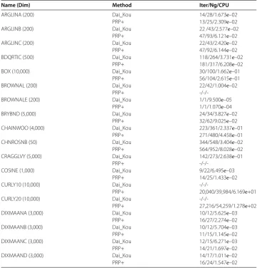
Figure 1 Performance profile for the test problems from the CUTEst library based on the number of iterations.

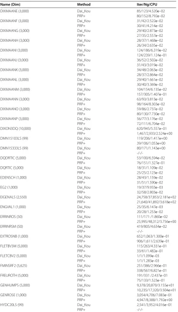
Figure 2 Performance profile for the test problems from the CUTEst library based on the number of gradient evaluations.

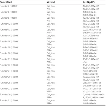
Figure 3 Performance profile for the test problems from the CUTEst library based on the CPU time.

Figure 5 Performance profile for some boundary value problems based on the number of gradient evaluations.

Figure 6 Performance profile for some boundary value problems based on the CPU time.

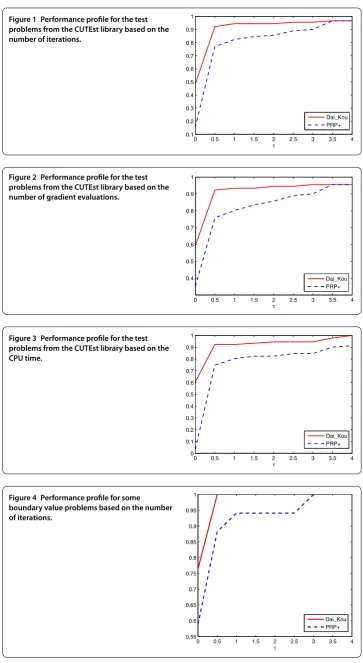
tions exceeded , or the gradient function generated ‘NaN’. The performances of the two methods were evaluated using the profiles of Dolan and Morè []. That is, we plotted the fraction P of the test problems for which each of the two methods was within a factorτ. In the performance profiles, the top curve represents the most robust one within the same factorτ, and the left curve represents the fastest one to solve the same percentage of test problems. Figures - show the performance profiles for test problems from the CUTEst library relating to the number of iterations, the number of gradient evaluations and the CPU time, respectively. Figures - show the performance profiles for some boundary value problems. These figures reveal that, for the test problems, the proposed method is more efficient and robust than the PRP+ conjugate gradient method. Consequently, the improved method not only can solve problems only referring to gradient information but also inherits the good numerical performance of the Dai-Kou type conjugate gradient methods.

5 Conclusions

nonlinear equation

F(x) =  ()

withF=g. While the convergence analysis of this paper needed some assumptions of the functionf whose gradient isg, our further investigation is to avoid the functionf and to solve general nonlinear equation () using different strategies from those of this paper and literature [–].

Competing interests

The authors declare that they have no competing interests.

Authors’ contributions

All authors read and approved the final version of this paper.

Acknowledgements

The authors are very grateful to the associate editor and reviewers for their valuable suggestions which have greatly improved the paper. This work was partially supported by the National Natural Science Foundation of China (No. 11471102) and the Key Basic Research Foundation of the Higher Education Institutions of Henan Province (No. 16A110012).

Publisher’s Note

Springer Nature remains neutral with regard to jurisdictional claims in published maps and institutional affiliations.

Received: 17 August 2016 Accepted: 22 March 2017

References

1. Fletcher, R, Reeves, C: Function minimization by conjugate gradients. Comput. J.7, 149-154 (1964)

2. Hestenes, MR, Stiefel, EL: Methods of conjugate gradients for solving linear systems. J. Res. Natl. Bur. Stand.49(5), 409-436 (1952)

3. Polak, E, Ribière, G: Note sur la méthodes de directions conjuguées. Rev. Fr. Inform. Rech. Opér., Sér Rouge16, 35-43 (1969)

4. Polyak, BT: The conjugate gradient methods in extreme problems. USSR Comput. Math. Math. Phys.9, 94-112 (1969) 5. Dai, YH, Yuan, Y: A nonlinear conjugate gradient method with a strong global convergence property. SIAM J. Optim.

10(1), 177-182 (1999)

6. Liu, Y, Storey, C: Efficient generalized conjugate gradient algorithms. Part 1: theory. J. Optim. Theory Appl.69, 129-137 (1991)

7. Dai, YH, Kou, CX: A nonlinear conjugate gradient algorithm with an optimal property and an improved Wolfe line search. SIAM J. Optim.23, 296-320 (2013)

8. Hager, WW, Zhang, HC: Algorithm 851: CG__DESCENT, a conjugate gradient method with guaranteed descent. ACM Trans. Math. Softw.32, 113-137 (2006)

9. Hager, WW, Zhang, HC: A new conjugate gradient method with guaranteed descent and an efficient line search. SIAM J. Optim.16, 170-192 (2005)

10. Zhang, L, Li, JL: A new globalization technique for nonlinear conjugate gradient methods for nonconvex minimization. Appl. Math. Comput.217, 10295-10304 (2011)

11. Nakamura, W, Narushima, Y, Yabe, H: Nonlinear conjugate gradient methods with sufficient descent properties for unconstrained optimization. J. Ind. Manag. Optim.9, 595-619 (2013)

12. Spedicato, E, Huang, Z: Numerical experience with Newton-like methods for nonlinear algebraic systems. Computing 58, 69-89 (1997)

13. Dong, YD: A practical PR+ conjugate gradient method only using gradient. Appl. Math. Comput.219, 2041-2052 (2012)

14. Powell, MJD: Convergence properties of algorithms for nonlinear optimization. SIAM Rev.28, 487-500 (1986) 15. Dong, YD: The BFGS method only using gradient. Preprint.

http://www.optimization-online.org/DB_FILE/2016/07/5560.pdf

16. Dai, YH, Liao, LZ: New conjugacy conditions and related nonlinear conjugate gradient methods. Appl. Math. Optim. 43, 87-101 (2001)

17. Lewis, AS, Overton, ML: Nonsmooth optimization via quasi-Newton methods. Math. Program.141(1-2), 135-163 (2013)

18. Zoutendijk, G: Nonlinear programming, computational methods. In: Abadie, J (ed.) Integer and Nonlinear Programming, pp. 37-86. North-Holland, Amsterdam (1970)

19. Bongartz, I, Conn, AR, Gould, N, Toint, PL: CUTE: constrained and unconstrained testing environment. ACM Trans. Math. Softw.21, 123-160 (1995)

20. Gould, NIM, Orban, D, Toint, PL: CUTEr and SifDec: a constrained and unconstrained testing environment, revisited. ACM Trans. Math. Softw.29, 373-394 (2003)

22. Dolan, ED, Morè, JJ: Benchmarking optimization software with performance profiles. Math. Program.91, 201-213 (2002)

23. Solodov, MV, Svaiter, BF: A globally convergent inexact Newton method for systems of monotone equations. In: Fukushima, M, Qi, L (eds.) Reformulation: Nonsmooth, Piecewise Smooth, Semismooth and Smoothing Methods, pp. 355-369. Kluwer Academic, Dordrecht (1999)

24. Yan, QR, Peng, XZ, Li, DH: A globally convergent derivative-free method for solving large-scale nonlinear monotone equations. J. Comput. Appl. Math.234, 649-657 (2010)