Volume 2010, Article ID 325654,14pages doi:10.1155/2010/325654
Research Article
A Parameter Robust Method for Singularly
Perturbed Delay Differential Equations
Fevzi Erdogan
Department of Mathematics, Faculty of Sciences, Yuzuncu Yil University, 65080 Van, Turkey
Correspondence should be addressed to Fevzi Erdogan,[email protected]
Received 29 April 2010; Revised 9 July 2010; Accepted 17 July 2010
Academic Editor: Alexander I. Domoshnitsky
Copyrightq2010 Fevzi Erdogan. This is an open access article distributed under the Creative Commons Attribution License, which permits unrestricted use, distribution, and reproduction in any medium, provided the original work is properly cited.
Uniform finite difference methods are constructed via nonstandard finite difference methods for the numerical solution of singularly perturbed quasilinear initial value problem for delay differential equations. A numerical method is constructed for this problem which involves the appropriate Bakhvalov meshes on each time subinterval. The method is shown to be uniformly convergent with respect to the perturbation parameter. A numerical example is solved using the presented method, and the computed result is compared with exact solution of the problem.
1. Introduction
Delay differential equations are used to model a large variety of practical phenomena in the biosciences, engineering and control theory, and in many other areas of science and technology, in which the time evolution depends not only on present states but also on states at or near a given time in the pastsee, e.g.,1–4. If we restrict the class of delay differential equations to a class in which the highest derivative is multiplied by a small parameter, then it is said to be a singularly perturbed delay differential equation. Such problems arise in the mathematical modeling of various practical phenomena, for example, in population dynamics4, the study of bistable devices 5, description of the human pupil-light reflex 6, and variational problems in control theory 7. In the direction of numerical study of singularly perturbed delay differential equation, much can be seen in8–16.
important to develop suitable numerical methods for these problems, whose accuracy does not depend on the perturbation parameter, that is, methods that are uniformly convergent with respect to the perturbation parameter17–20.
In order to construct parameter-uniform numerical methods for singularly perturbed differential equations, two different techniques are applied. Firstly, the fitted operator approach20which has coefficients of exponential type adapted to the singular perturbation problems. Secondly, the special mesh approach19, which constructs meshes adapted to the solution of the problem.
The work contained in this paper falls under the second category. We use the nonstandard finite difference methods originally developed by Bakhvalov for some other problems. One of the simplest ways to derive such methods consists of using a class of special meshes such as Bakhvalov meshes; see, e.g.,18–24, which is constructed a priori and depend on the perturbation parameter, the problem data, and the number of corresponding mesh points.
In this paper, we study the following singularly perturbed delay differential problem in the intervalI 0,T:
εut atut ft, ut−r, t∈I, 1.1
ut ϕt, t∈I0, 1.2
whereI 0, T mp1Ip,Ip {t : rp−1 < t ≤ rp}, 1 ≤ p ≤ m,andrs sr, for 0 ≤ s ≤ m
andI0 −r,0. 0< ε≤1 is the perturbation parameter, andr >0 is a constant delay, which
is independent ofε.at,ϕt,andft, vare given sufficiently smooth functions satisfying certain regularity conditions inIandI×R, respectively moreover
at≥α >0, ∂f ∂v
≤M <∞. 1.3
The solution,ut, displays in general boundary layers on the right side of each point t rs0≤s≤mfor small values ofε.
In the present paper we discretize 1.1-1.2 using a numerical method which is composed of an implicit finite difference scheme on special Bakhvalov meshes for the numerical solution on each timesubinterval. InSection 2, we state some important properties of the exact solution. In Section 3, we describe the finite difference discretization and introduce Bakhvalov-Shishkin mesh and Bakhvalov mesh. In Section 4, we present the error analysis for the approximate solution. Uniform convergence is proved in the discrete maximum norm. InSection 5, a test example is considered and a comparison of the numerical and exact solutions is presented.
In the works of Amiraliyev and Erdogan 9, special meshesShishkin mesh have been used. The method that we propose in this paper uses Bakhvalov-type meshes.
2. The Continuous Problem
Before defining the mesh and the finite difference scheme, we show some results about the behavior with respect to the perturbation parameter of the exact solution of problem 1.1-1.2 and its derivatives, which we will use in later section for the analysis of an appropriate numerical solution. For any continuous functiongt,g∞denotes a continuous maximum norm on the corresponding closed intervalI; in particular we will useg∞,p
maxI
p|gx|,0≤p≤m.
Lemma 2.1. The solutionutof the problem1.1-1.2satisfies the following estimates:
u∞,p ≤Cp, 1≤p≤m, 2.1
where
Cpϕ∞,0
1 α−1Mp α−1
p
s1
1 α−1Mp−sF∞,p, p1,2, . . . , m,
Ft ft,0,
2.2
u≤C ⎧ ⎨ ⎩1
t−rp−1
p−1
εp exp
−α
t−rp−1
ε
⎫⎬
⎭, t∈Ip, 1≤p≤m, 2.3
provided
∂f∂t≤C, fort∈I, |v| ≤C0, 2.4
where
C0ϕ∞,0
1 α−1Mm α−1F∞,I1 α−1Mm−1
. 2.5
Proof. The quasilinear equation1.1can be written in the form
εut atut btut−r Ft, t∈I, 2.6
where
bt −∂f ∂vt,v,
vγut−r 0< γ <1-intermediate values.
Applying the maximum principle onIpgives
u∞,p ≤urp−1 α−1
b∞,pu∞,p−1 F∞,p
≤1 α−1Mu
∞,p−1 α−1F∞,p,
2.8
which implies the first-order difference inequality
wp≤μwp−1 ψp, 2.9
with
wpu∞,p, μ1 α−1M, ψpα−1F∞,p. 2.10
From the last inequality, it follows that
wp≤w0μp p
s1
μp−sψs 2.11
which proves2.1.
Now we prove2.3. The proof is verified by induction. Forp1.it is known that
ut≤C
1 1
εexp
−αt
ε
. 2.12
Now, let2.3hold true forpk. Differentiating1.1, we have the relation forpk 1
εut atut gt, t∈Ik 1, 2.13
where
gt −ut∂a ∂t
∂f
∂tt, ut−r ∂f
∂vt, ut−ru
t−r. 2.14
Then, from2.13we have the following relation forut:
ut urkexp
−1
ε
t
rk
asds
1
ε
t
rk
gτexp
−1
ε
t
τ
asds
dτ. 2.15
Using the estimate2.3forpkandttk, we have
urk≤C
1 r
k−1
εk exp
−αr
ε
Hence,
ur
k≤C, k≥1. 2.17
Furthermore, using now2.3forpk, we get
gt≤ut∂a ∂t
∂f∂tt, ut−r ∂f
∂vt, ut−r
ut−r
≤C1 ut−r
≤C
1 t−rk
k−1
εk exp
−αt−rk
ε
.
2.18
Taking into account2.17and2.18in2.15, we have
ut≤Cexp
−
αt−rk
ε
1
εC
t
rk
1 τ−rk
k−1
εk exp
−
ατ−rk
ε
exp
−
αt−τ ε
dτ
≤C Ct−rk ε α
−1ε
1−exp
−αt−rk
ε
1
εCexp
−αt−rk
ε
t−rkk
kεk
≤C
1 t−rk
k
εk 1 exp
−
αt−rk
ε
, t∈Ik 1,
2.19
which proves2.3.
3. Discretization and Mesh
LetωN0be any nonuniform mesh onI
ωN0{0t0< t1<· · ·< tN0 T, τiti−ti−1} 3.1
which contains byNmesh point at each subintervalIp1≤p≤m
ωN,p
ti:
and consequently,
ωN0
m
p1
ωN,p. 3.3
To simplify the notation, we setgi gtifor any functiongt; moreover,yidenotes
an approximation ofutatti. For any mesh function{wi}defined onωN0, we use
wt,i wi−wi−1 τi
,
w∞,N,pw∞,ωN,p : max
p−1N≤i≤pN|wi|, 1≤p≤m.
3.4
For the difference approximation to1.1, we integrate1.1overti−1, ti
εut,i τ−1
ti
ti−1
atutdtτ−1
ti
ti−1
ft, ut−rdt, 3.5
which yields the relation
εut,i aiui Rifti, ui−N, 1≤i≤N0, 3.6
with the local truncation error
Ri−τi−1
ti
ti−1
t−ti−1d
dtatut
dt
−τ−1 i
ti
ti−1
ti−1−t
d
dtft, ut−r
dt.
3.7
As a consequence of 3.6, we propose the following difference scheme for approximation to1.1-1.2:
εyt,i aiyifti, ui−N, 1≤i≤N0,
yiϕi, −N≤i≤0.
3.8
3.1. Bakhvalov-Shishkin Mesh
Let us introduce a non-uniform meshωN,p which will be generated as follows. For the even
numberN, the non-uniform meshωN,pdivides each of the intervalrp−1,σpandσp,rpinto
N/2 subintervals, where the transition pointσp, which separates the fine and coarse portions
of the mesh is defined by
σprp−1 α−1θpεlnN, 1≤p≤m, 3.9
whereθ1 ≥ 1 andθp > 12 ≤ p ≤ mare some constants. We will assume throughout the
paper thatε≤N−1, as is generally the case in practice.
Hence, ifτpdenote the step sizes inσp, rp, we have
τp2
rp−σp
N−1, 1≤p≤m. 3.10
The corresponding mesh points are
ti ⎧ ⎪ ⎪ ⎪ ⎪ ⎨ ⎪ ⎪ ⎪ ⎪ ⎩
rp−1−α−1θpε ln
1−
1−N−12i
N
, ip−1N, . . . ,
p−1
2
N,
σp
i− N
2
τp, i
p−1
2
N 1, . . . , pN, 1≤p≤m.
3.11
3.2. Bakhvalov Mesh
In order the difference scheme3.8, to beε-uniform convergent, we will use the fitted form of
ωN,p. This is a special non-uniform mesh which is condensed in the boundary layer. The fitted
special non-uniform meshωN,p on the intervalrp−1, rpis formed by dividing the interval
into two subintervalsrp−1, σpandσp, rp, where
σprp−1−α−1θpεlnε, 1≤p≤m. 3.12
In practice one usually hasσp ≤ rp. So, the mesh is fine onrp−1, σpand coarse on
σp, rp. The corresponding mesh points are
ti ⎧ ⎪ ⎪ ⎪ ⎪ ⎨ ⎪ ⎪ ⎪ ⎪ ⎩
rp−1−α−1θpεln 1−
1−ε2i N
!
, ip−1N, . . . ,
p−1
2
N,
σp
i−N
2
τp, i
p−1
2
N 1, . . . , pN, 1≤p≤m.
4. Stability and Convergence Analysis
To investigate the convergence of the method, note that the error functionziyi−ui, 0≤i≤
N0, is the solution of the discrete problem
εzt,i aizi Rif
ti, yi−N
−fti, ui−N, 1≤i≤N0,
ziϕi, −N≤i≤0,
4.1
where the truncation errorRiis given by3.7.
Lemma 4.1. Letyibe an approximate solution of1.1-1.2. Then, the following estimate holds
y∞,ω
N,p≤ϕ∞,ωN,0
1 α−1Mp α−1 p
k1
f∞,ω
N,k
1 α−1Mp−1, 1≤p≤m. 4.2
Proof. The proof follows easily by induction inp, by analogy with differential case.
Lemma 4.2. Letzibe the solution of 4.1. Then, the following estimate holds:
z∞,N,p≤C
p
k1
R∞,ωN,k, 1≤p≤m. 4.3
Proof. It evidently follows from4.2by takingϕ≡0 andf ≡R.
Lemma 4.3. Under the above assumptions ofSection 1andLemma 2.1, for the error functionRi, the
following estimate holds:
R∞,ωN,p≤CN−1, 1≤p≤m. 4.4
Proof. From explicit expression3.7forRi, on an arbitrary mesh, we have
|Ri| ≤τi−1
ti
ti−1
t−ti−1
dtdatut−ft, ut−rdt, 1≤i≤N0. 4.5
This inequality together with2.1enables us to write
|Ri| ≤C
τi
ti
ti−1
ut ut−rdt
From here, in view of2.3, it follows that
|Ri| ≤C
τi 1
ε
ti
ti−1
e−αt/εdt
, for 1≤i≤N, 4.7
|Ri| ≤C
⎧ ⎨ ⎩τi
ti
ti−1
t−rp−1
p−1
εp e−
αt−rp−1/εdt
ti
ti−1
t−rp−1
p−2
εp−1 e
−αt−rp−1/εdt
⎫ ⎬ ⎭,
for ti∈Ip
p >1.
4.8
Applying the inequalityxke−x≤Ce−γx, 0< γ <1,x∈0,∞to4.7, we deduce
|Ri| ≤C
τi 1
ε
ti
ti−1
e−αt−rp−1/θpεdt
, forti∈Ip, θp>1, p >1. 4.9
Combining4.7and4.9, we can write
|Ri| ≤C
τi
1
ε
ti
ti−1
e−αt−rp−1/θpεdt
, forti∈Ip, p1,2, . . . , m, θ1≥1, θp>1
p≥2 4.10
where
τi τp,
p−1
2
N 1≤i≤pN. 4.11
At each submeshωN,p,we estimate the truncation errorRi for Bakhvalov-Shishkin
mesh as follows. We estimateRi onrp−1, σpandσp, rpseparately. We consider thatti ∈
σp, rp. We obtain from4.10that
|Ri| ≤C
"
τp α−1θp
e−αti−1−rp−1/θpε−e−αti−rp−1/θpε
#
C"τp α−1θpN−1e−αi−1−p−1/2Nτp/θpε
1−e−ατp/θpε#.
4.12
This implies that
|Ri| ≤CN−1. 4.13
On the other hand, in the layer regionrp−1, σp,4.10becomes
|Ri| ≤C
"
τi α−1θp
Hereby, since
τiti−ti−1
α−1θpε
−ln
1−
1−N−12i
N
ln
1−
1−N−12i−1
N
≤2α−1θpε
1−N−1≤CN−1,
4.15
e−αti−1/ε−e−αti/ε 21−N−1N−1 4.16
then
|Ri| ≤4α−1θpCN−1,
p−1N≤i≤
p−1
2
N, 1≤p≤m. 4.17
We estimate the truncation errorRifor Bakhvalov mesh as follows. We consider first
ti∈σp, rp. Inσp, rp; that is, outside the layer|ut| ≤Cand|ut−r| ≤Cε−pe−αt/ε≤1by
2.1and4.7. Hereby, we get from4.7and4.10that
|Ri| ≤Cτi,
p−1N≤i≤
p−1
2
N. 4.18
Hence,
|Ri| ≤2CrN−1,
p−1N≤i≤
p−1
2
N. 4.19
Next, we estimateRiforrp−1, σp.
Since
τiti−ti−1
α−1θpε
−ln 1−1−ε2i
N
!
ln 1−1−ε2i−1
N
!
≤2α−1θp1−εN−1,
4.20
e−αti−1/ε−e−αti/ε21−εN−1, 4.21
recalling thatε≤N−1, it then follows from4.12that
|Ri| ≤4α−1θpCN−1. 4.22
Thus, the proof is completed.
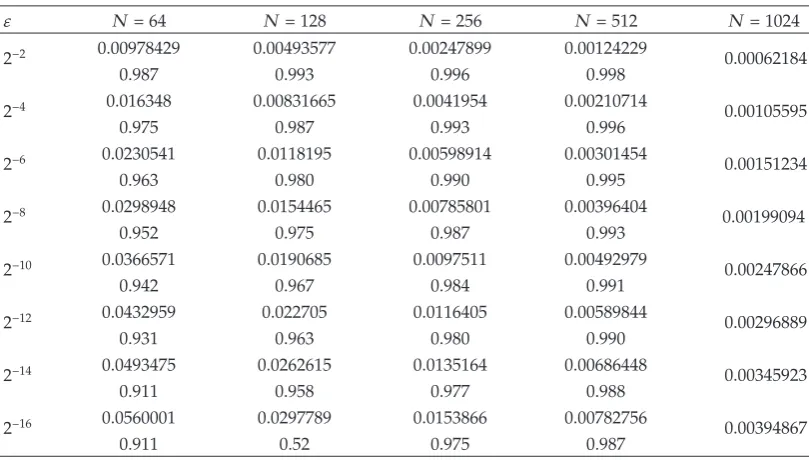
Table 1:Maximum Errors and Rates of Convergence for the Bakhvalov-Shishkin Mesh onωN,1.
ε N64 N128 N256 N512 N1024
2−2 0.00978429 0.00493577 0.00247899 0.00124229 0.00062184
0.987 0.993 0.996 0.998
2−4 0.016348 0.00831665 0.0041954 0.00210714 0.00105595
0.975 0.987 0.993 0.996
2−6 0.0230541 0.0118195 0.00598914 0.00301454 0.00151234
0.963 0.980 0.990 0.995
2−8 0.0298948 0.0154465 0.00785801 0.00396404 0.00199094
0.952 0.975 0.987 0.993
2−10 0.0366571 0.0190685 0.0097511 0.00492979 0.00247866
0.942 0.967 0.984 0.991
2−12 0.0432959 0.022705 0.0116405 0.00589844 0.00296889
0.931 0.963 0.980 0.990
2−14 0.0493475 0.0262615 0.0135164 0.00686448 0.00345923
0.911 0.958 0.977 0.988
2−16 0.0560001 0.0297789 0.0153866 0.00782756 0.00394867
0.911 0.52 0.975 0.987
Theorem 4.4. Letube the solution of 1.1-1.2, and letybe the solution of 3.8. Then, for both meshes the following estimate holds:
y−u
∞,ωN,p ≤CN
−1, 1≤p≤m, 4.23
whereCis a constant independent ofNandε.
5. Numerical Results
We begin with an example from Driver2for which we possess the exact solution
εut ut ut−1, t∈0, T,
ut 1 t, −1≤t≤0.
5.1
The exact solution for 0≤t≤2 is given by
ut
⎧ ⎪ ⎪ ⎪ ⎨ ⎪ ⎪ ⎪ ⎩
−ε t 1 εe−t/ε, t∈0,1,
−1−2ε t 1 εe−t/ε ε−1
ε
1 1
ε
t
!
e1−t/ε, t∈1,2.
Table 2:Maximum Errors and Rates of Convergence for the Bakhvalov-Shishkin Mesh onωN,2.
ε N64 N128 N256 N512 N1024
2−2 0.0120441 0.00609088 0.00306261 0.00153567 0.00076893
0.983 0.991 0.995 0.997
2−4 0.0204344 0.0106567 0.00542574 0.0027399 0.00137664
0.939 0.973 0.985 0.992
2−6 0.0206243 0.0123374 0.00663473 0.00346693 0.00178218
0.741 0.894 0.936 0.960
2−8 0.0251094 0.0129806 0.00660313 0.00346667 0.00192158
0.951 0.975 0.929 0.951
2−10 0.0308922 0.0160402 0.00819434 0.00414173 0.00208219
0.945 0.968 0.992 0.996
2−12 0.0358208 0.0190729 0.00978373 0.00495569 0.00249403
0.909 0.963 0.981 0.990
2−14 0.0418982 0.0220722 0.0113657 0.00576776 0.00290598
0.924 0.957 0.978 0.988
2−16 0.0471824 0.0250121 0.0129303 0.00657754 0.0033174
0.915 0.951 0.975 0.987
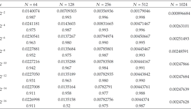
Table 3:Maximum Errors and Rates of Convergence for the Bakhvalov Mesh onωN,1.
ε N64 N128 N256 N512 N1024
2−2 0.0140074 0.00709303 0.00356936 0.00179046 0.000896684
0.987 0.993 0.996 0.998
2−4 0.0241181 0.0143603 0.00831665 0.00471467 0.00263101
0.975 0.987 0.993 0.996
2−6 0.0230541 0.0137267 0.00794974 0.00450667 0.00251493
0.963 0.980 0.990 0.995
2−8 0.0227881 0.0135684 0.00785801 0.00445467 0.00248591
0.952 0.975 0.987 0.993
2−10 0.0227216 0.0135288 0.00783508 0.00444167 0.00247866
0.942 0.967 0.984 0.991
2−12 0.0227050 0.0135189 0.00782935 0.00443842 0.00247684
0.931 0.963 0.980 0.990
2−14 0.0227008 0.0135164 0.0782791 0.00443761 0.00247639
0.911 0.958 0.977 0.988
2−16 0.0226998 0.0135158 0.00782756 0.0044374 0.00247628
0.911 0.52 0.975 0.987
We define the computed parameter-uniform maximum erroreN,pε as follows:
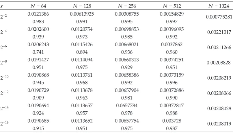
[image:12.600.99.503.387.618.2]Table 4:Maximum Errors and Rates of Convergence for the Bakhvalov Mesh onωN,2.
ε N64 N128 N256 N512 N1024
2−2 0.0121386 0.00613925 0.00308755 0.00154829 0.000775281
0.983 0.991 0.995 0.997
2−4 0.0202600 0.0120754 0.00698853 0.00396095 0.00221017
0.939 0.973 0.985 0.992
2−6 0.0206243 0.0115426 0.00668021 0.0037862 0.00211266
0.741 0.894 0.936 0.960
2−8 0.0191427 0.0114094 0.00660313 0.00374251 0.00208828
0.951 0.975 0.929 0.951
2−10 0.0190868 0.0113761 0.00658386 0.00373159 0.00208219
0.945 0.968 0.992 0.996
2−12 0.0190729 0.0113678 0.00657904 0.00372886 0.00208066
0.909 0.963 0.981 0.990
2−14 0.0190694 0.0113657 0.0657784 0.00372817 0.00208028
0.924 0.957 0.978 0.988
2−16 0.0190685 0.0113652 0.00657754 0.003728 0.00208019
0.915 0.951 0.975 0.987
whereyis the numerical approximation toufor various values ofN, ε. We also define the computed parameter-uniform rate of convergence to be
rN,p ln
eN,p/e2N,p
ln 2 , p1,2. 5.4
The values ofεfor which we solve the test problem areε2−i, i2,4, . . . ,16. Tables1,2,3,
and4verify theε-uniform convergence of the numerical solution on both subintervals, and computed rates are essentially in agreement with our theoretical analysis.
References
1 R. Bellman and K. L. Cooke,Differential-Difference Equations, Academic Press, New York, NY, USA, 1963.
2 R. D. Driver,Ordinary and Delay Differential Equations, vol. 2 ofApplied Mathematical Sciences, Springer, New York, NY, USA, 1977.
3 A. Bellen and M. Zennaro,Numerical Methods for Delay Differential Equations, Numerical Mathematics and Scientific Computation, Oxford University Press, Oxford, UK, 2003.
4 Y. Kuang,Delay Differential Equations with Applications in Population Dynamic, vol. 191 ofMathematics in Science and Engineering, Academic Press, Boston, Mass, USA, 1993.
5 S.-N. Chow and J. Mallet-Paret, “Singularly perturbed delay-differential equations,” in Coupled Nonlinear Oscillators, J. Chandra and A. C. Scott, Eds., pp. 7–12, North-Holland, Amsterdam, The Netherlands, 1983.
6 A. Longtin and J. G. Milton, “Complex oscillations in the human pupil light reflex with mixed and delayed feedback,”Mathematical Biosciences, vol. 90, no. 1-2, pp. 183–199, 1988.
7 M. C. Mackey and L. Glass, “Oscillation and chaos in physiological control systems,”Science, vol. 197, no. 4300, pp. 287–289, 1977.
9 G. M. Amiraliyev and F. Erdogan, “A finite difference scheme for a class of singularly perturbed initial value problems for delay differential equations,”Numerical Algorithms, vol. 52, no. 4, pp. 663– 675, 2009.
10 J. Mallet-Paret and R. D. Nussbaum, “A differential-delay equation arising in optics and physiology,” SIAM Journal on Mathematical Analysis, vol. 20, no. 2, pp. 249–292, 1989.
11 J. Mallet-Paret and R. D. Nussbaum, “Multiple transition layers in a singularly perturbed diff erential-delay equation,”Proceedings of the Royal Society of Edinburgh A, vol. 123, no. 6, pp. 1119–1134, 1993.
12 S. Maset, “Numerical solution of retarded functional differential equations as abstract Cauchy problems,”Journal of Computational and Applied Mathematics, vol. 161, no. 2, pp. 259–282, 2003.
13 B. J. McCartin, “Exponential fitting of the delayed recruitment/renewal equation,” Journal of Computational and Applied Mathematics, vol. 136, no. 1-2, pp. 343–356, 2001.
14 M. K. Kadalbajoo and K. K. Sharma, “ε-uniform fitted mesh method for singularly perturbed differential-difference equations: mixed type of shifts wtih layer behavior,”International Journal of Computer Mathematics, vol. 81, no. 1, pp. 49–62, 2004.
15 H. Tian,Numerical treatment of singularly perturbed delay differential equations, Ph.D. thesis, Department of Mathematics, University of Manchester, 2000.
16 H. Tian, “The exponential asymptotic stability of singularly perturbed delay differential equations with a bounded lag,” Journal of Mathematical Analysis and Applications, vol. 270, no. 1, pp. 143–149, 2002.
17 E. P. Doolan, J. J. H. Miller, and W. H. A. Schilders,Uniform Numerical Methods for Problems with Initial and Boundary Layers, Boole Press, Dublin, Ireland, 1980.
18 P. A. Farrell, A. F. Hegarty, J. J. H. Miller, E. O’Riordan, and G. I. Shishkin,Robust Computational Techniques for Boundary Layers, vol. 16 ofApplied Mathematics, Chapman & Hall/CRC, Boca Raton, Fla, USA, 2000.
19 J. J. Miller, E. ORiordan, and G. I. Shishkin,Fitted Numerical Methods for Singular Perturbation Problems, Error Estimates in the Maximum Error for Linear Problems in One and Two Dimensions, World Scientific, Singapore, 1996.
20 H.-G. Roos, M. Stynes, and L. Tobiska,Numerical Methods for Singularly Perturbed Differential Equations: Convection-Diffusion and Flow Problems, vol. 24 ofSpringer Series in Computational Mathematics, Springer, Berlin, Germany, 1996.
21 N. S. Bakhvalov, “Towards optimization of methods for solving boundary value problems in the presence of boundary layers,”Zhurnal Vychislitelnoi Matematiki I Matematicheskoi Fiziki, vol. 9, pp. 841–859, 1969Russian.
22 N. Kopteva, “Uniform pointwise convergence of difference schemes for convection-diffusion problems on layer-adapted meshes,”Computing, vol. 66, no. 2, pp. 179–197, 2001.
23 T. Linss, “Analysis of a Galerkin finite element method on a Bakhvalov-Shishkin mesh for a linear convection-diffusion problem,”IMA Journal of Numerical Analysis, vol. 20, no. 4, pp. 621–632, 2000.