“0” and “O” Recognition Based on Deep Learning

2019 International Conference on Computer Intelligent Systems and Network Remote Control (CISNRC 2019) ISBN: 978-1-60595-651-0

“0” and “O” Recognition Based on Deep Learning

Wuyi Xiao, Junxian Ma, Huazhu Liu and Chunping Liao

ABSTRACT

The traditional algorithm has achieved good recognition for the recognition of most characters, but the recognition rate of the number “0” and the letter “O” is only 80-90%, which is difficult to meet the actual needs of the industry. For the recognition of these two characters, a recognition method based on deep learning is proposed. First, image preprocessing is performed on the characters, and then the sample data is manually labeled, and 40,000 training samples and 10,000 test sample images are obtained by the data samples enhancement. The results show that the CNN network can achieve more than 99% recognition rate, the training sample time is about 5 minutes, and 1000 images can be recognized in 1 second. Both the recognition speed and the recognition effect can meet the actual needs of the industry.

KEYWORDS

Number “0”, The Letter “O”, Deep Learning, CNN Network.

INTRODUCTION

Prior to the advent of deep learning, the mainstream algorithms were the connected region-or HOG-based detection methods that were based on the traditional handcraft features[1][2]. For example, the candidates for characters were de- rived through the maximally stable extremal regions (MSER), which were then regarded as the vertex of the graph.

At this time, the search for text lines could be considered as a process of clustering, since the texts from the same lines were usually identical in direction, color, font, and shape.

T. Siriteerakul et al.[3] empirically studied the classification of ThaiCEnglish characters by using SVM [4] classifier with HOG features. Despite large numbers of characters of different classes, their method performed adequately well under some identifiable defects. The 2D graphic-based contour projection and morphological processing proposed by Chhaya Patel et al.[5] showed an accuracy of up to 89.24% for segmentation of handwritten text words. Chhaya Patel et al.[6] _________________________________________

Wuyi Xiao, Junxian Ma, Huazhu Liu, Chunping Liao

School of Electronics & Information Engineering Shenzhen University

School of Electrical Engineering & Intelligentization Dong Guan University of Technology Shenzhen, China

proposed a Euclidean transformation-based region recognition method, whose accuracy for region recognition of handwritten text words reached 96.99%. S. Mandal et al.[7] put forward a frequent counting-based method utilizing the first, second derivatives and the slope and baseline characteristics, which showed an accuracy of 95.1% for handwritten character recognition. The accuracy rate of a SVM-based approach proposed by H. Nakkach et al.[8] was 92.43% for the identification and classification of Arabic characters. The deep learning-based convolutional neural network put forward by Shuye Zhang et al.[9] exhibited an accuracy of 98.44% for the recognition classification of similar Chinese characters.

The first step of conventional methods was image preprocessing, where the original image samples were processed to obtain the characters needing recognition, so that the subsequent feature extraction and learning could be performed. The primary purpose of this step was to remove redundant information from the sample images to better facilitate the subsequent processing. This process usually includes: grayscaling (for color sample images), denoising[10], binarization[11], character segmentation, and normalization. After binarization, the sample images only have two gray values of 0 and 255; among which 0 is the image background and 255 is the character under recognition. Denoising is vitally important at this stage, where the quality of noise reduction algorithm has a great influence on the feature extraction. Character segmentation divides the characters in an image into single characters that need recognition. Often, an additional slant correction will be required if the characters are slanted. In normalization operation, single character images are resized to the same size. A unified algorithm can be applied only under the same specification. Feature extraction (via various methods, e.g. PCA[12], or SIFT[13]): Features are key information used to identify characters, and each individual character can be distinguished from others by features. The SIFT-based off-line handwritten Chinese character recognition function proposed by Zhiyi Zhang et al.[14] could achieve a recognition rate of over 95%, which though failed to meet the expected level for hardly identifiable features. The classifier design, training, and recognition constitute the final step in character recognition. Classifiers[15] and[16] are used to perform recognition. For a character image, features are extracted as input to the classifiers, which then identify and classify these features.

Most of the industrial optical character recognition (OCR) techniques performed recognition detection based on traditional methods before the introduction of deep learning AlexNet[17]. However, the classification accuracy for the hard-to-distinguish “0” and “O” characters with the traditional recognition methods was undesirable after feature extraction. Therefore, deep learning CNN[18] [19] [20] [21] network model was used for their feature extraction, followed by training and test recognition with classifier, which improved the accuracy considerably (99% or higher).

RELATED WORK

tation of original datasets to obtain the training samples. Furthermore, the training samples are labeled, and a dataset is created and denoted as tfrecord. The second module is the CNN network, which extracts feature vectors from each training sample image. The third module is a set of SoftMax[22].

ACQUISITION AND READING OF SAMPLE SETS

The core problem of identifying 0-O by deep learning training can be summarized, firstly, as about the sample quantity: the industrially acquired original images are 500 in number, which is rather small. For the training identification of small sample sets, an increase of samples is necessary. In this study, the dataset is increased by data enhancement[6]. For example, flipping, random trimming, color dithering, translation transformation, scale transformation, contrast transformation, noise perturbation, and rotation transformation/reflection transformation of images each adds 10 sample datasets to obtain 50,000 sample images in total. The second core problem faced by the training is the data reading mode. The length of training is decided largely by the way the data is read during training. Three methods of data reading are compared under the same sample training conditions. The first method is to read each training sample image, where the placeholder reads the data in the memory, and then feeds them to the holder variable via feed dict for value passing. The second method is to read the data in the hard disk by using queue. The third method is to prepare the data into tfrecord datasets before reading them using queue. In the GPU1080ti-based condition[23], training 10,000 steps with 5,000 training samples by method one took more than 5 hours, while with method three, only 250 seconds were consumed. The use of method three for data reading can address the time wastage caused by the training duration in the course of learning or engineering training. Table I lists the comparison of training durations:

TABLE I. COMPARISON OF TRAINING TIME BETWEEN THREE DATA READING METHODS.

Methods Method 1 Method 2 Method 3

Training time (secs) 19080 954 250

IMAGE PREPROCESSING

Figure 2. For the cut single characters, we extract the “0” and “O” we need, thereby obtaining the desired training dataset samples. This is the end of character segmentation part. After character extraction, the extracted character matrix is normalized into 64*64 matrix. Next, the segmented 0-O sample images are labeled and made into tfrecord datasets, as shown in Figure 3.

Figure 1. Original single images (500 in number).

Figure 2. Segmentation of single images in Figure 1.

Figure 3. Labeling of 0-O two types of data.

Data reading is performed on the obtained datasets by queue method. The reading thread continuously reads the images in the file system into a memory queue, while another thread is responsible for calculation. Data are read directly from the memory queue when required by the calculation. A queue is not just a data structure, which can also be an important mechanism for calculating the tensor value in one step. For example, multiple threads are able to simultaneously write elements to a queue or read elements in a queue. This can solve the idle GPU problem attributed to IO, thereby generating batches, which are then input into the CNN network for training.

DEEP LEARNING ALGORITHM

combines all local features into global features, which are used for calculating the scores for each of the last classes. Activation function introduces nonlinearity into the CNN.

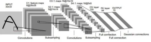
Taking the LeNet-5 network[24] as an example, as shown in Figure. 4, the first hidden layer is convolved, which comprises six feature maps. Each feature map consists of 28*28 neurons, and each neuron specifies a 5*5 acceptance domain. The second hidden layer implements subsampling and local averaging, which also comprises 6 feature maps, except that each feature map consists of 14*14 neurons. The third hidden layer, which performs second convolution, comprises 16 feature maps, each consisting of 10*10 neurons. The fourth hidden layer, which is responsible for the second subsampling and local averaging calculation, comprises 16 feature maps, but each consisting of 5*5 neurons. The fifth hidden layer implements the last stage of convolution, which consists of 120 neurons, with each specifying a 5*5 acceptance domain. Finally, the fully- connected layer obtains the output class vectors.

Figure 4. Structure schematic of LeNet-5 network.

EXPERIMENTS

The CNN part adopts a LeNet5 network structure, in view of its relatively moderate training duration and number of training network layers.

DESCRIPTION OF VARIOUS LENET-5 NETWORK PARTS

• Input: 64*64 = 4,096 0-O character images, equivalent to 4,096 neurons. These character images contain the number 0 and the letter O, which equal to two categories of images.

• C1 layer: 16 feature convolution kernels are selected, whose size is 5*5, so that we can get 16 feature maps each with a size of 64-5+1=60. That is, the number of neurons is 16*60*60= 57600.

• S2 layer: Downsampling layer, which performs down-sampling by maximum

pooling. The pooling filter size f is selected as (2, 2), whereas the stride is 2. This way, we can get 16 images each with an output size of 30*30.

• C3 layer: Convolutional layer, the size of convolution kernels remains 5*5,

according to which we can derive a new image size of 30-5+1=26. Since 16 convolution kernels are adopted here, 16 images sized 26 * 26 are output finally.

• S4 layer: Downsampling layer, which performs maximum pooling on the 16

• C5 layer: The output of S4 layer is tiled into a 2704 one- dimensional vector.

Then, the next layer is constructed with these 2,704 neurons. The C5 layer contains 120 neurons. The 2,704 neurons in the S4 layer are connected to each neuron in the C5 layer (120 in total) to constitute the fully-connected layer, which can be regarded as a standard neural network layer.

• F6 layer: Another fully-connected layer is added to the C5 layer’s 120 neurons (the F6 layer contains 128 neurons).

• Output: Finally, the F6 layer’s 128 neurons are fed into a SoftMax function to

derive a tensor with an output length of 2. The position 1 in the tensor represents the category.

SOFTMAX

Softmax regression model is a generalization of the logistic regression model concerning the multi-classification problem. For the multi-classification problem, the number of classes to be classified is greater than 2, and the classes are mutually exclusive. After the completion of convolutional, pooling, and fully-connected layers and data conversion to sample label space, binary classification of input images is needed (that is, we hope to calculate the conditional probability of each class conditioned by this image, a prior probability distribution). A column vector of length 2 can be derived via the fully- connected layer, which is a linear predictor generated by the network. Softmax is precisely a common function in machine learning for converting linear predictors into output probabilities, which is used to output the conditional probabilities for each class.

ANALYSIS OF EXPERIMENTAL RESULTS

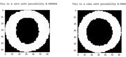
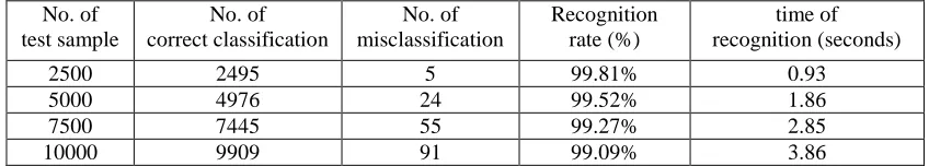
The experiments reveal a recognition rate of 99.83% for testing the number “0” alone; and a recognition rate of 99.71% for testing the letter “O” alone. The experimental results are shown in Figure 5, respectively. TABLE II lists the comparison of recognition rate and time. The recognition of 10,000 long images takes only 3.86 seconds, with a recognition rate of 99.09%. Compared to the references [5-9], not only the recognition rate is improved greatly, but the recognition duration is also shorter, which can fully meet the online recognition requirements.

TABLE II. TABLE TYPE STYLES. No. of

test sample

No. of correct classification

No. of misclassification

Recognition rate (%)

time of recognition (seconds)

2500 2495 5 99.81% 0.93

5000 4976 24 99.52% 1.86

7500 7445 55 99.27% 2.85

10000 9909 91 99.09% 3.86

CONCLUSION

In this paper, the training samples are obtained by pre- processing of the original sample images primarily from the field of computer vision, especially the deep learning. The sample dataset reading method greatly shortens the duration of convolutional network training. By combining the computer vision with the classical deep learning tool (CNN), an excellent recognition rate can be attained effectively for characters with hard-to-distinguish features. The experiments show that the deep learning-based recognition can reach an accuracy of over 99%. Besides, the training time is also shortened greatly by changing the way data is read. The application of methods based on such data reading mode and deep learning is expected to be ever mature for the recognition of various more hard-to- distinguish characters.

ACKNOWLEDGMENT

This work was supported by the Science and Technology Project of Guangdong Province under Grand No. 2017B010132001 and 2016A010101038.

REFERENCES

1. D. Scherer, A. Miller, and S. Behnke, “Evaluation of pooling operations in convolutional architectures for object recognition”, International Conference on Artificial Neural Networks, 2010.

2. N. Dalal and B. Triggs. Histograms of oriented gradients for human detection. In CVPR, 2005. 3. T. Siriteerakul. Mixed thai-english character classification based on histogram of oriented

gradient feature. In 2013 12th International Conference on Document Analysis and Recognition, pages 847C851, Aug 2013.

4. P. F. Felzenszwalb, R. B. Girshick, D. McAllester, and D. Ramanan, “Object detection with discriminatively trained part-based models”, IEEE Trans. Pattern Anal. Mach. Intell, vol. 32, no. 9, pp. 1627-1645, 2010.

5. Chhaya Patel and Apurva Desai, “Segmentation of text lines into words for Gujarati handwritten text”, International conference on Signal and Image Processing, pp. 130-134, 2010.

6. Chhaya Patel and Apurva Desai, “Zone Identification for Gujarati Hand- written Word”, Second international conference on Emerging application of Information technology, pp. 194-197, 2011.

7. S. Mandal, H. Choudhury, S. R. M. Prasanna, and S. Sundaram, “Frequency Count based Two Stage Classification for Online Handwritten Character Recognition”, International Conference on Signal Processing and Communications (SPCOM), 2016.

9. Shuye Zhang, Lianwen Jin, and Liang Lin, “Discovering similar Chinese characters in online handwriting with deep convolutional neural networks”, International Journal on Document Analysis and Recognition (IJDAR), vol. 19, no. 3, pp. 237-252, 2016.

10. Dabov, K. Foi, A. Katkovnik, and V. Egiazarian, “Image denoising by sparse 3-D transform-domain collaborative filtering”, IEEE Trans. Image Process., 2007, 16, (8), pp. 2080C2095. 11. N. Otsu, “A threshold selection method from gray-level histograms”, Automatica, vol. 11, no.

285C296, pp. 23-27, 1975.

12. J. Yang and D. Zhang, “Two-dimensional PCA: A new approach to appearance-based face representation and recognition”, IEEE Trans. Pattern Anal. Mach. Intell., vol. 26, no. 1, pp. 131C137, Jan. 2004.

13. D. Lowe. Distinctive image features from scale-invariant keypoints. IJCV, 2004.

14. Zhiyi Zhang, Lianwen Jin, Kai Ding, and Xue Gao. “Character-SIFT: a novel feature for offline handwritten Chinese character recognition”, 10th International Conference on Document Analysis and Recognition, 2009.

15. C. Cortes and V. Vapnik, Support-vector networks. Machine learning, vol. 20, no. 3, pp. 273-297, 1995.

16. V. N. Vapnik, The nature of statistical learning theory. New York, NY, USA: Springer-Verlag New York, Inc., 1995.

17. J. Deng, A. Berg, S. Satheesh, H. Su, A. Khosla, and L. Fei-Fei. ImageNet Large Scale Visual Recognition Competition 2012 (ILSVRC2012).

18. Karen Simonyan and Andrew Zisserman, “Very deep convolutional networks for large-scale image recognition”, Computer Science, 2014.

19. Yann Lecun, Yoshua Bengio, and Geoffrey Hinton, “Deep learning”, Nature, vol. 521, no. 7553, pp. 436-444, 2015.

20. R. Girshick, “Fast r-cnn”, Proceedings of the IEEE international conference on computer vision, pp. 1440-1448, 2015.

21. S. Ren, K. He, R. Girshick, and J. Sun, “Faster R-CNN: Towards real- time object detection with region proposal networks”, Advances in neural information processing systems, pp. 91-99, 2015.

22. Xingqun Qi, Tianhui Wang, and Jiaming Liu, “Comparison of Support Vector Machine and Softmax Classifiers in Computer Vision”, ICMCCE, 2017.

23. D. Strigl, K. Kofler, and S. Podlipnig, “Performance and scalability of GPU-based convolutional neural networks”, 18th Euromicro Conference on Parallel Distributed and Network-Based Processing, 2010.