Detection of multiple change points for linear processes under negatively super additive dependence

(1)

R E S E A R C H

Open Access

Detection of multiple change points for

linear processes under negatively

super-additive dependence

Yuncai Yu

1

_{, Xinsheng Liu}

1*

_{, Ling Liu}

2

_{and Piao Zhao}

1

*_{Correspondence:}

[email protected]

1_{State Key Laboratory of Mechanics}

and Control of Mechanical Structures, Institute of Nano Science and Department of Mathematics, Nanjing University of Aeronautics and Astronautics, Nanjing, China Full list of author information is available at the end of the article

Abstract

This paper focuses on the issue of detecting the multiple change points for linear processes under negatively super-additive dependence (NSD). We propose a CUSUM-type method in the multiple variance change model and establish the weak convergence rate of the change points estimation. To carry out this method, we give a multiple variance-change iterative (MVCI) algorithm. Additionally, some simulations are implemented to substantiate the validity of the CUSUM-type method.

Comparison with some best methods indicates that the CUSUM-type change point estimation is computationally competitive and superior in terms of the mean squared error (MSE).

MSC: 62F03; 62F05; 62F12

Keywords: Multiple change points; Linear processes under NSD; Variance change; CUSUM-type estimation; Weak convergence rate

1 Introduction

As a common feature of ‘big data’, change point arises in many areas such as signal process-ing (Basseville [1]), ﬁnance (Chen and Gupta [2]), ecology (Hawkins [3]), disease outbreak watch (Sparks et al. [4]), and neuroscience (Ratnam et al. [5]; Lena et al. [6]) and has been much investigated in the last few decades. To detect change point and estimate its lo-cation, there has emerged a number of approaches including least squares (LS, Bai [7]), Bayesian method (Fearnhead [8]), maximum likelihood (Zou et al. [9]), and some non-parametric methods (Matteson and James [10]; Haynes et al. [11]). The cumulative sum (CUSUM) method, based on the LS estimation, is a very attractive one for detecting the variance change in a sequence because it avoids some assumptions about the underlying error distribution function and is computed simply (Gombay et al. [12]). For independent sequences, Gombay et al. [12] constructed the CUSUM statistic to detect and estimate the change of variance. Wang and Wang [13] used the CUSUM test to detect the vari-ance change in a linear process with long memory errors. Zhao et al. [14] considered the ratio test for variance change in a linear process. Qin et al. [15] investigated the strong convergence rate of the CUSUM estimator of the variance change in linear processes.

However, most of the references above assume the change point number in a sequence is one, which is a serious restriction when applied to practical problems. For multiple change

(2)

point detection, Inclán and Tiao [16] employed the cumulative sums of squares to detect the multiple changes of variance in the uncorrelated sequences. Lavielle [17] obtained the convergence rate for multiple change detection for strongly mixing and strongly depen-dent processes. Li and Zhao [18] gave the convergence rate for multiple change-points es-timation of moving-average processes. More recently, Haynes et al. [11] proposed a com-putationally eﬃcient nonparametric approach for change point detection, and Laurentiu et al. [19] oﬀered the Bayesian loss-based approach to analyze change point problem. But both of them require the information of the underlying error distribution function, which may lead to the complexity of computation.

In this contribution, we consider the following multiple variance change model:

Yt=μ+σiet, ti∗–1≤t≤t∗i, 1≤i≤r, (1)

whereris the known number of change points,μandσi(1≤i≤r) are parameters,t∗i, 1≤i≤r,t∗₀= 0,t_r∗₊₁=nare the true change locations witht_i∗= [τin], where [x] denotes the integer part ofx,τ= (τ₁∗,τ₂∗, . . . ,τ_r∗) are the change points, andet is linear processes given as follows:

et= ∞

j=0

ajεt–j, (2)

where aj is an array of real numbers satisfying

∞

j=0a2j <∞, {εm,m∈Z} are stationary random variables.

Under the independent or dependent assumptions of{εm,m∈Z}, the convergence rates of the single change point estimators have been established for the linear processes (2). We refer to Bai [7] and Qin et al. [15] for independence case, to Li and Zhao [18] for linear negative quadrant dependence, and to Wang and Wang [13] for long range dependence. In this article, we will consider the multiple variance change model, and simultaneously {εm,m∈Z}are negatively super-additive dependence (NSD) whose deﬁnition is based on the super-additive functions.

Deﬁnition 1(Hu [20]) A functionφis called super-additive if

φ(x∨y) +φ(x∧y)≥φ(x) +φ(y)

for allx,y∈Rn, where “∨” is componentwise maximum and “∧” represents component-wise minimum.

Deﬁnition 2(Hu [20]) A random vector (X1,X2, . . . ,Xn) is said to be NSD if

Eφ(X1,X2, . . . ,Xn)≤Eφ

X₁∗,X₂∗, . . . ,X_n∗, (3)

(3)

Deﬁnition 3 (Wang et al. [21]) A sequence of random variables (X1,X2, . . . ,Xn, . . .) is called NSD if, for alln≥1, (X1,X2, . . . ,Xn) is NSD.

NSD has received considerable attention since it includes the well-known negative asso-ciation (see Christoﬁdes and Vaggelatou [22]). Eghbal et al. [23] explored the strong law of large numbers and the rate of convergence for NSD sequences with the existence of high order moments. Shen et al. [24] and Wu et al. [25] got the almost sure and complete con-vergence, respectively, for NSD random variables. Wang et al. [26] investigated the com-plete convergence, and Yu et al. [27] established the central limit theorem for weighted sums of NSD random variables. Moreover, NSD samples have been introduced to various models; for example, under NSD errors, Yu et al. [27] considered the M-test problem of regression parameters in a linear model; Wang et al. [28] studied the strong consistency and weak consistency of the LS estimators in an EV regression model, and Yu et al. [29] obtained the convergence rates of the wavelet thresholding estimators in a nonparametric regression model.

The aim of this study is to detect the multiple change points for linear processes under NSD. We propose the CUSUM-type change point estimator in model (1) and establish the weak convergence rate of the estimator with the mean parameterμestimated by its LS estimator. Moreover, some simulations are implemented byR Softwareto compare the CUSUM-type estimator with some methods. The result indicates that the CUSUM-type change point estimator is broadly comparable with those obtained by the typical methods. The remainder of this paper is organized as follows. In Sect.2, we describe the CUSUM-type multiple change point estimation and give the weak convergence rate of this estima-tor. Also, we give a multiple variance-change iterative (MVCI) algorithm to evaluate the estimator. In Sect.3, some simulations are presented to show the performances of the estimator. Finally, the proofs of the main results are given in Sect.4.

2 Estimation and main results

LetY˜j=Yj–μˆn, whereμˆn=1_n

n

t=1Ytis the LS estimator of the meanμ. Assume that

An,r=

(t0,t1, . . . ,tr+1),t0= 0 <t1<· · ·<tr<tr+1=n

is a set of allowable r-partitions. We further consider the following set of allowabler -partitions:

Aδn

n,r=

(t0,t1, . . . ,tr+1) :ti–ti–1≥nδn

,

whereδnis a non-increasing non-negative sequence satisfyingδn→0 andnδn→ ∞. For eachti, 1≤i≤r+ 1, we deﬁne

R(ti) =

(ti–ti–1)(ti+1–ti) (ti+1–ti–1)2

1

ti–ti–1 ti

t=ti–1+1 ˜

Y_t2– 1

ti+1–ti ti+1

t=ti+1

˜

Y_t2 .

Denoteτˆδn₌ˆ_tδn

/n, the CUSUM-type multiple change point estimator is given by

ˆ

τδn

=arg max

t∈Aδn n,r

1

n

r+1

i=1

(4)

To derive our results, we list several conditions as follows.

(A1) {εm,m∈Z}are stationary NSD random variables withEεm= 0and

Var(εm) =σ2<∞.

(A2) For alll≥1, we have_m_:_|l_–_m|≥u|Cov(εl,εm)| →0, asu→ ∞. (A3) Eε4

m<∞holds for allm≥1. (A4) ∞_j₌₀|aj|<∞.

Remark1 Conditions (A1) and (A2) are easily satisﬁed (see Yu et al. [29]). (A3) is often ap-plied to obtain the convergence rate of change point estimator (e.g., Qin et al. [15]; Shi et al. [30]). Condition (A4) is weaker than Bai [11], which requires∞_j₌₀j|aj|<∞. Furthermore, condition (A4) implies that∞_j₌₀a2

j <∞and

∞

j=0a4j <∞.

Theorem 1 Assume that conditions(A1)–(A4)hold.Then,for all1≤j≤r,we have

ˆ

τδn

j →τj∗, in probability.

When the meanμis known, Qin et al. [15] established the strong convergence of the CUSUM estimator. It is obvious that Theorem1is still true whenμis known, and we will give the following corollary without proof.

Corollary 1 If the mean is known(μ= 0),conditions(A1)–(A4)hold,then we have the same conclusion of Theorem1.

Under assumptions (A1)–(A4), we can further establish the convergence rate of the CUSUM-type multiple change point estimatorτˆδn

.

Theorem 2 Let M(n)be a natural number sequence with M(n)→ ∞.Then,under the conditions of Theorem1,we further have

ˆ

τδn

j –τj∗=o

M(n)/n, in probability.

To implement the CUSUM-type multiple change-point method, we also give the multi-ple variance-change iterative (MVCI) algorithm based on Qin et al. [15] and Shi et al. [30] as follows:

Step 1.Chooseη≥1, computeμˆnand{ ˜Yt2}.

Step 2. Seti= 1,m= 0, andl= [nδn]. Divide the sample intoLsubintervalsIjwith the equal interval lengthl.

Step 3. For each subintervalIj,j= 1, 2, . . . ,L, ﬁndˆt(ji)=arg maxt∈(1+m,m+l)R(tj).

Step 4. Compute the set={R(tˆ_j(i))}, and selectrchange locations which correspond to

rmaximum values ofR(ˆt_j(i)) in the set.

Step 5. For the selected r change locations ˆt_j(i), j = 1, . . . ,r, ﬁnd ˆt(_ji+1) =

arg max_t∈

(tˆ(_ji)–2M(l),tˆ_j(i+1)+2M(l))R(tj).

Step 6. Setl= 4M(l) andm=ˆt(_ji)– 2M(l).

Step 7. Ifˆt(i+1)–tˆ(i)_∞<η, then proceed to Step 8, otherwise seti=i+ 1, go back to Step 3.

Step 8.ˆtMVCI=tˆ (i)

andτˆMVCI=ˆt (i)

(5)

3 Simulation studies

We present a set of simulation studies to illustrate the availability of the CUSUM-type MVCI algorithm via R packages. Additionally, we implement some available competitors including segment neighborhood (SN), pruned exact linear time (PELT), binary segmenta-tion (BS), and wild binary segmentasegmenta-tion (WBS) to compare the performance of the MVCI algorithm.

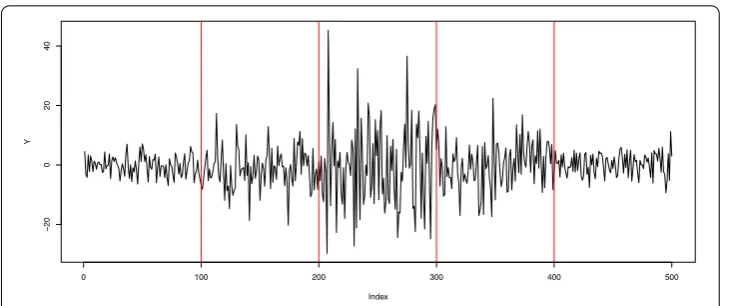
In model (1), we taker= 4,μ= 0,σ1= 2,σ2= 4,σ3= 8,σ4= 4,σ5= 2, and suppose the true change locationst∗₁ = 100,t∗₂= 200, t₃∗= 300,t₄∗= 400, we model the NSD se-quence{εm,m∈Z}as a multivariate mixture of normal distribution with joint distribu-tionN(0, 0, 1, 4; –0.5). The sample size is taken to ben= 500 and the weight functions are satisﬁedaj= 2–j,j∈Z. Figure1displays the simulated sequence ofYt, 1≤t≤500, and the true change locations.

To carry out the SN (Auger and Lawrence [31]), PELT (Killick et al. [32]), BS (Killick and Eckley [33]), we use the penalty likelihood method, which can be implemented by change-pointpackage in (Killick [34]). As to WBS (Killick and Eckley [33]), we utilize package

wbsts(Korkas, Karolos, and Piotr [35]) in our model with the thresholdλn=C √

2log1/2n, where C= 1. We assume the parameter δn=n–1/2 in the MVCI algorithm. The mean squared error (MSE) of the CUSUM-type variance change point estimator ofτ∗is deﬁned as MSE = 1_rr_i₌₁(τˆi–τi∗)

2

, and the performances of the above methods are described in Table1(all of the simulations are run for 100 replicates).

Table 1presents the average MSEs of the MVCI, SN, PELT, BS, and WBS methods. Generally, the ﬁrst change point is overestimated and the rest change points are underesti-mated. When the sample size is large (n= 500), all of the methods can estimate the change points availably, but the MVCI method is superior in terms of the average MSE. This also

[image:5.595.117.482.446.599.2]

Figure 1The simulated time sequence ofYt, the red vertical lines are true change locations

Table 1 Comparison of the MVCI algorithm with SN,PELT, BS, and WBS methods

τi∗ n SN PELT BS WBS MVCI

0.2 500 0.222 0.222 0.218 0.210 0.210

0.4 500 0.410 0.398 0.392 0.406 0.396

0.6 500 0.590 0.590 0.594 0.590 0.592

0.8 500 0.784 0.792 0.796 0.792 0.790

[image:5.595.118.480.658.732.2]

(6)

indicates that the CUSUM-type variance-change method is computationally competitive with some of best change point estimation methods.

4 Proof of the theorems

Throughout the proof, letCbe a general positive constant andc0,c1,c2,C0,C1, . . . ,C4be some positive constants. Denotex+₌_xI₍_x_≥_{0) and}_x–_{= –}_xI₍_x_{< 0). In the following we} will state some lemmas which are needed.

Lemma 1(Hu [20]) An NSD random sequence{Xm,m≥1}possesses the following prop-erties.

(P1) For anyx1,x1, . . . ,xn,

P(X1≤x1,X2≤x2, . . . ,Xn≤xn)≤ n

m=1

P(Xm≤xm).

(P2) {–X1, –X2, . . . , –Xn}is also NSD.

(P3) Letf1,f2, . . .be a sequence of non-decreasing Borel functions,then{fn(Xn),n≥1}is

still an NSD random sequence.

Lemma 2(Wang et al. [21]) Suppose that{Xm,m≥1}is an NSD random sequence with EXm= 0and E|Xm|α<∞for someα≥2,then for all n,

E

max

1≤k≤n

k

m=1

Xm

α ≤C

_n

m=1

E|Xm|α+

_n

m=1

EX2_m α/2

.

Lemma 3 Suppose that{Xm,m≥1}is an NSD random sequence with conditions(A1)–

(A2)hold,{am, 1≤m≤n,n≥1}is a sequence of real numbers satisfying

_∞

m=1a2m<∞.

Then

σ_n2=Var

_∞

m=1

amεn–m

≤Cσ2.

Proof For a pair of NSD random variablesX,Y, by property (P1) in Lemma1, we have

H(x,y) =P(X≤x,Y≤y) –P(X≤x)P(Y≤y)≤0.

The covariance ofXandYis veriﬁed to be negative by

Cov(X,Y) =E(XY) –E(X)E(Y) = H(x,y)dx dy≤0. (5)

Then, foru≥1,

l,m=1,|l–m|≥u

_a_l_a_mCov(Xl,Xm)

≤

l=1

m=l+u

(7)

≤ l=1

a2_l

m=l+u

Cov(Xl,Xm)+ m=u+1

a2_m

m–u

l=1

Cov(Xl,Xm)

≤

l=1

a2_l

|m–l|≥u

Cov(Xl,Xm)

≤sup

l

m=1,|l–m|≥u

|Cov(Xl,Xm)|

m=1

a2_m

.

Hence, by condition (A2), for a ﬁxed smallε> 0, there exists a positive integeru=uεsuch that

l,m=1,|l–m|≥u

alamCov(Xl,Xm)≤ε.

SetK= [1/ε] andYm=

u(m+1)

l=um+1alXl,m= 0, 1, . . . ,n,

Υm=

l: 2Km≤l≤2Km+K,Cov(Yl,Yl+1)≤ 2

K

2Km+K

l=2Km

Var(Ym)

.

Deﬁneh0= 0,hm+1=min{h:h>hm,h∈Υm}, and put

Zm= hm+1

l=hm+1

Yl, m= 0, 1, . . . ,n,

Λm=

u(hm+ 1) + 1, . . . ,u(hm+1+ 1)

.

Note that

Zm=

l∈Λm

alXl, m= 0, 1, . . . ,n.

It is easy to see that#Λm≤3Ku, where#stands for the cardinality of a set. From Lemma2, it follows that

σ_n2 =E

m=1

Z2_m+

1≤m<l≤n

Cov(Zm,Zl)

=

m=1

E

l∈Λm

alXl

2

+

1≤m<l≤n,|m–l|=1

Cov(Zm,Zl)

+

1≤m<l≤n,|m–l|>1

Cov(Zm,Zl)

≤

m=1

a2_mE

l∈Λm

Xl

2

+

m=1

Cov(Yhm,Yhm+1)

+

1≤m<l≤n,|m–l|≥u

|amal|Cov(Zm,Zl)

≤

m=1

l∈Λm

a2_lE(Xl)2+ 1

K

m=1

(8)

≤ m=1

l∈Λm

a2_lE(Xl)2+u

K

m=1

l∈Λm

a2_lE(Xl)2+ε

≤

m=1

E(amXm)2+

Cu K

m=1

E(amXm)2+ε=Cσ2,

which completes the proof of Lemma3.

Lemma 4 Suppose that etis linear processes under NSD random sequence with conditions (A1)–(A4)hold,letσ_ε2=E(e2

t).Then

E

_k

t=1

e2_t –σ_ε2

2

≤Ck.

Proof According to Lemma3, we obtain

σ_ε2=E

_∞

j=0

ajεt–j

2

≤Cσ2<∞.

Obviously, there exists a positive numberc0such that

e2_t –σ_ε2= ∞

j=0

a2_jε_t2_–_j–c0σ2

+ 2

0≤s<l<∞

asalεt–sεt–l.

Hence

Ee2_t –σε2

2 =E

_∞

s=0

a2_sε2_t_–_s–c0σ2

2

+ 4E

0≤s<l<∞

asalεt–sεt–l

2

+ 4E

_∞

l=0

a2_lε2_t_–_l–c0σ2

0≤s<l<∞

=E

_∞

s=0

a4_sε2_t_–_s–c0σ2

2

+ 2E

0≤s<l<∞

a2_la2_sε2_t_–_l–c0σ2

ε2_t_–_s–c0σ2

+ 4E

0≤s<l<∞

asalεt–sεt–l

+ 4E

_∞

j=0

0≤s<l<∞

a2_jasal

ε2_t_–_s–c0σ2

εt–sεt–l

≤Eε_j2–c0σ2

2∞

s=0

a4_s+ 4

0≤s<l<∞

a2_sa2_lEε2_t_–_sε2_t_–_l

=:H1+H2.

By conditions (A3) and (A4), we obtain

H1≤C

Eε4_t – 2c0σ2Eε2t +c20σ4

(9)

Decomposingεt asεt =εt+–ε–t, from properties (P2) and (P3) in Lemma1, one can see thatε+_t,ε–_t, (ε_t–)2 _{and (}_ε+

t)2 are NSD random sequences. From formula (5), we have

E(XY)≤E(X)E(Y), then

H2= 4

0≤s<l<∞

a_s2a2_lEε_t+_–_s–ε–_t_–_s2ε_t+_–_l–ε_t–_–_l2

≤4

0≤s<l<∞

a2_sa2_lEε_t+_–_s2+ε_t–_–_s2·ε_t+_–_l2+ε–_t_–_l2

≤16

0≤s<l<∞

a2_sa2_lσ4<∞. (7)

Combining (6) and (7), we get

Ee2_t –σ_ε22<∞. (8)

Now we consider the cross term. For anyt<j, one can see that

Ee2_t –σ_ε2e2_j –σ_ε2

=E

_∞

s=0

a2 s

ε_t2_–_s–σ2+ 2 0≤s<l<∞

·

_∞

s=0

a2_sε2_j_–_s–c0σ2

+ 2

0≤s<l<∞

asalεt–sεj–l

=E

_∞

s=0

a2_sε_t2_–_s–c0σ2

· ∞

˜ s=0

a2_sε_t2_–_s–σ2

+ 2 ∞

s=0

a2_sε_t2_–_s–c0σ2

0≤s_<_l_<_∞

asalεt–sεj–l

+ 2E

_∞

s=0

a2_sε2_t_–_s–c0σ2 0≤s<l<∞

+ 4E

0≤s<l<∞

asalεj–sεj–l

= ∞

s=0 ∞

s=0

a2_sa2_sEεt2–s–c0σ2

ε_t2_–_s–c0σ2

+ 2 s=0

0≤s<l<∞

a2_sasalE

ε2_t_–_s–c0σ2

ε_j2_–_sε_j2_–_l

+ 2 ∞

s=0

0≤s<l<∞

a2_sasalE

ε2_t_–_s–c0σ2

εt–sεt–l

+ 4

0≤s<l<∞

(10)

Lets=j–t+s,l=j–t+l, similar to the proof of inequality (8), we have

Ee2_t –σ_ε2e2_j –σ_ε2

= ∞

s=0

a2_sa2_j_–_t₊_sEε_t2_–_s–c0σ2

2

+ 4

0≤s<l<∞

asalaj–t+saj–t+lE(εt–sεt–l)2<∞.

Hence

1≤t<j≤k

Ee2_t–σ_ε2e2_j–σ_ε2

=

1≤t<j≤k

E

ε2_t –c0σ2

2∞

s=0

a2_sa2_j_–_t₊_s+ 4σ2

0≤s<l<∞

asalaj–t+saj–t+l

≤Cσ4

k–1

t=1 k

j=t+1 ∞

s=0

a2_sa2_j_–_t₊_s+ 4σ4

k–1

t=1 k

j=t+1

0≤s<l<∞

|asalaj–t+saj–t+l|

=C _k_–1 t=1 ∞ s=0

a2_s

k

j=t+1

a2_j_–_t₊_s+ k–1

t=1

0≤s<l<∞

|asal| k

j=t+1

|aj–t+saj–t+l|

≤C k _∞ s=0

a2_s 2 +k _∞ s=0 as

2_∞

u=0

a2_u

≤Ck.

Lemma 5 Let Y1,Y2, . . . ,Ynbe a sample from model(1),assume thatY˜t=Yt–μˆn,μˆn= 1

n

t=1Yt,if assumptions(A1)–(A4)hold,then for anyε> 0,

P max 1≤k≤n 1 k k t=1 _˜

Y_t2–EY˜_t2 >ε

≤√C

n.

Proof Note that

k

t=1

˜

Y_t2= k

t=1

σ_i2e2_t– 2(μˆn–μ) k

t=1

σ_i2e2_t+k(μˆn–μ)2,

whereet= (Yt–μ)/σi, then

P max 1≤k≤n 1 k k t=1 _˜

Y_t2–EY˜_t2 >ε ≤P max 1≤k≤n

σ_i2

k k t=1

e2_t –Ee2_t > ε 3

+P(μˆn–μ)2–E(μˆn–μ)2>

ε 3 +P max 1≤k≤n

σ_i2

k

2(μˆn–μ) k

t=1

e2_t – 2E(μˆn–μ) k

t=1

e2_t > ε 3

(11)

Applying Lemma 4, it is easy to see that J1 ≤C/√n. From Markov’s inequality, J2 is bounded by

J2 =P

σ_i2

1 n n t=1 et 2 –E 1 n n t=1 et 2 > ε 3

≤ 3σi2

ε E 1 n n t=1 et 2 –E 1 n n t=1 et 2

≤ 6σi2

ε E 1 n n t=1 et 2 ≤C n.

Now, we will show thatJ3≤C/

√

n. By Cauchy–Schwarz’s inequality, it follows

max

1≤k≤nE

(μˆn–μ)

1

k

t=1

σiet

≤σ_i2 max

1≤k≤n E 1 n n t=1 et

21/2

max 1≤k≤n E 1 k k t=1 et

21/2

≤√C

n. Therefore P max 1≤k≤n 1 k

2(μˆn–μ) k

t=1

σiet

> ε 6 ≤P max 1≤k≤n _k t=1 et 2 +1 k _k t=1

e2_t

>

ε

6σ_i2

≤P max 1≤k≤n _k t=1 et 2 > ε

12σ2 i +P max 1≤k≤n 1 k _k t=1

e2_t

> ε 12σ2

i

≤_√c1

n+ c2 n ≤ C √ n.

Thus the proof of Lemma5is completed.

Proof of Theorem1 Letδ0= (σi2–σi2–1)

∞

j=0a2j, forti≤ti∗, we have

ER(ti)

=(ti–ti–1)(ti+1–ti) (ti+1–ti–1)2

E

1

ti–ti–1 ti

t=ti–1+1 ˜

Y_t2– 1

ti+1–ti ti+1

t=ti+1

˜

Y_t2

=(ti–ti–1)(ti+1–ti) (ti+1–ti–1)2

E

1

ti–ti–1 ti

t=ti–1+1 ˜

Y_t2– 1

ti+1–ti t_i∗

t=ti+1

˜

Y_t2– 1

ti+1–ti ti+1

t=t∗_i+1

˜

Y_t2

=(ti–ti–1)(ti+1–ti) (ti+1–ti–1)2

σi2–1

∞

j=0

a2_j – t ∗ i –ti

ti+1–ti

σ_i2_–1

∞

j=0

a2_j –ti+1–t ∗ i

ti+1–ti

σ_i2

∞

j=0

(12)

=(ti–ti–1)(ti+1–ti) (ti+1–ti–1)2

(ti+1–t∗i)

ti+1–ti |δ0|

=(ti–ti–1)(ti+1–t ∗ i) (ti+1–ti–1)2

|δ0|.

Similarly, forti≥ti∗,

ER(ti)

=(ti–ti–1)(ti+1–ti) (ti+1–ti–1)2

E

1

ti–ti–1 t∗_i

t=ti–1+1 ˜

Y_t2+ 1

ti–ti–1 ti

t=t∗_i+1

˜

Y_t2– 1

ti+1–ti ti+1

t=t_i∗+1

˜

Y_t2

=(ti–ti–1)(ti+1–ti) (ti+1–ti–1)2

t_i∗–ti

ti+1–ti

σ_i2_–1

∞

j=0

a2_j+ ti–t ∗ i

ti–ti–1

σ_i2

∞

j=0

a2_j –σ_i2

∞

j=0

a2_j

=(ti+1–ti)(t ∗ i –ti–1) (ti+1–ti–1)2

|δ0|.

Note thatER(ti) is increasing forti≤ti∗decreasing whileti≥t∗i, thus the maximum of

ER(ti) is

ERt_i∗=(ti+1–t ∗

i)(t∗i –ti–1) (ti+1–ti–1)2

|δ0|.

By direct calculation, it follows

ERt_i∗–ER(ti)≥

(t_i∗–ti–1)∧(ti+1–t∗i) (ti+1–ti–1)2

ti–t∗i|δ0| ≥

C0

n ti–t

∗

i=C0τi–τi∗. In order to prove Theorem1, it is desired to show that, for anyε> 0,

Pτˆ–τ∗_∞≥ε→0.

Since R(ti) = R(ti) – ER(ti) + (ER(ti) – R(ti∗)) + R(ti∗) and |R(ti∗) –ER(ti∗)| ≤

max_t∈Aδn

n,r|R(ti) –ER(ti)|, then

R(ti)–Rti∗≤R(ti) –ER(ti)+R

ti∗

–ERti∗+ER(ti) –ER

ti∗

≤2max

t∈Aδn n,r

R(ti) –ER(ti)+ER(ti) –ERti∗

.

DeﬁneΛn,r={t∈Aδnn,r,t–t∗∞≥nε}, then

Pτˆ–τ∗_∞≥ε≤P

max

t∈Λn,r

r

i=1

_R₍_t_i)–Rt_i∗≥0

≤P

2max

t∈Λn,r

r

i=1

R(ti) –ER(ti)– r

i=1

C0τˆ–τ∗_∞≥0

≤P

max

1≤i≤rR(ti) –ER(ti)≥δ

(13)

where δ=C0ε/2 is an arbitrarily small positive number. According to the deﬁnition of

ER(ti), one can see that

max

1≤i≤rR(ti) –ER(ti)

= max

1≤ti–1<ti<ti+1≤n

(ti–ti–1)(ti+1–ti) (ti+1–ti–1)2

1

ti–ti–1 ti

t=ti–1+1

_˜

Y_t2–EY˜_t2

– 1

ti+1–ti ti+1

t=ti+1 _˜

Y_t2–EY˜_t2

≤ max

1≤ti–1<ti≤n

1

ti–ti–1

ti

t=ti–1+1

_˜

Y_t2–EY˜_t2

+ max

1≤ti<ti+1≤n

1

ti+1–ti

ti+1

t=ti+1 _˜

Y_t2–EY˜_t2

. (10)

From (9) and (10), the proof of Theorem1will be completed by showing

P

max

1≤ti–1<ti≤n

1

ti–ti–1

ti

t=ti–1+1

_˜

Y_t2–EY˜_t2 >δ

→0, n→ ∞, (11)

and

P

max

1≤ti<ti+1≤n

1

ti+1–ti

ti+1

t=ti+1 _˜

Y_t2–EY˜_t2 >δ

→0, n→ ∞. (12)

Since Eq. (12) can be proved similarly as (11), we only consider Eq. (11), thus the proof of Theorem1is ﬁnished by takingk=ti–ti–1in Lemma5.

Proof of Theorem 2 Letθ be a constant in the interval (0, 1). DenoteDnM,r(n)={t∈Aδnn,r,

nθ>t–t∗_∞>M(n)}. By Theorem1, we have

Pτˆ–τ∗_∞>M(n)/n≤Pτˆ–τ∗_∞≥θ+Pθ>τˆ–τ∗_∞>M(n)/n

≤ε+P

max

t∈DM(n)

n,r

r

i=1

_R₍_t_i)–Rt∗_i≥0

.

Without loss of generality, we assume thatδ0< 0. In view of the fact that|x| ≥ |y|is equivalent to (i)x–y≥0 andx+y≥0, or (ii)x–y≤0 andx+y≤0, then

P

max

t∈DM(n)

n,r

r

i=1

R(ti)–R

t_i∗≥0

≤P

max

t∈DM(n)

n,r

r

i=1

R(ti) –Rt∗_i≥0

+P

max

t∈DM(n)

n,r

r

i=1

R(ti) +Rt_i∗< 0

≤P

max

t∈DM(n)

n,r ,ti<t∗i

r

i=1

R(ti) –Rt_i∗≥0

+P

max

t∈DM(n)

n,r ,ti≥t∗i

r

i=1

R(ti) –Rt_i∗≥0

(14)

+P

max

t∈DM(n)

n,r

r

i=1

R(ti) +Rt_i∗< 0

=:T1+T2+T3.

Forti<t∗i, we have

R(ti) –ER(ti) –Rt∗_i–ERt_i∗

≤ C1|ti–ti∗| (ti+1–ti–1)2

ti

t=ti–1+1

_˜

Y_t2–EY˜_t2 +

C2|ti–ti∗| (ti+1–ti–1)2

ti+1

t=t_i∗+1

_˜

Y_t2–EY˜_t2

+ C3

ti+1–ti–1

t∗_i

t=ti–1+1

_˜

Y_t2–EY˜_t2 +

C4

ti+1–ti–1

t∗_i

t=ti–1+1

_˜

Y_t2–EY˜_t2 .

Sinceδ0< 0,ER(ti)≥0, then for 1≤i≤r,

T1≤P

t∈DM(n)

n,r ,ti<t∗i

_r

i=1

R(ti) –ER(ti) –Rt∗_i–ERt∗_i≥

r

i=1

ERt∗_i–ER(ti)

≤P

t∈DM(n)

n,r ,ti<t∗i

_r

i=1

R(ti) –ER(ti) –Rt∗_i–ERt∗_i

≥ r i=1 C0 t∗_i –ti

/(ti+1–ti–1)

≤P

max

nδn≤ti–ti–1≤n

1

ti+1–ti–1

ti

t=ti–1+1

_˜

Y_t2–EY˜_t2 ≥C1

+P

max

nδn≤ti–ti–1≤n

1

ti+1–ti–1

ti+1

t=t_i∗+1

_˜

Y_t2–EY˜_t2 ≥C2

+P

max

M(n)≤t∗i–ti≤θn

1

t∗_i –ti

t∗_i

t=ti–1+1

_˜

Y_t2–EY˜_t2 ≥C3

+P

max

M(n)≤t∗i–ti≤θn

1

t∗_i –ti

t∗_i

t=ti–1+1

_˜

Y_t2–EY˜_t2 ≥C4

=:Q1+Q2+Q3+Q4.

In the view ofnδn→ ∞andM(n)→ ∞, Lemma5yields

Qi→0, i= 1, 2, 3, 4.

ThusT1→0. We can treatT2analogously asT1, henceT2→0.

To complete the proof of Theorem2, it is suﬃcient to showT3→0. SinceR(ti) +R(ti∗)≤ 0 implies thatR(ti) –ER(ti) +R(ti∗) –ER(ti∗)≤–ER(ti) –ER(t∗i)≤–ER(t∗i), we obtain

(15)

According toER(t_i∗)≥0 (δ0< 0), inequality (13) implies that

R(ti) –ER(ti)≥ER

t∗_i/2 or Rt∗_i–ERt_i∗≥ERt∗_i/2.

Hence

T3≤P

t∈DM(n)

n,r

r

i=1

_R₍_t_{i) –}_ER₍_t_i)_≥_ER t_i∗/2

+P

t∈DM(n)

n,r

r

i=1

_R

t_i∗–ERt_i∗≥ERt∗_i/2

≤2P

t∈DM(n)

n,r

r

i=1

R(ti) –ER(ti)≥ERt_i∗/2

≤2rP

max

1≤i≤rR(ti) –ER(ti)≥ER

t∗_i/2

.

Combining (4), (5), (6), and (7), we get

P

max

1≤i≤r

R(ti) –ER(ti)≥ERt_i∗/2

→0.

ThusT3→0. This completes the proof of Theorem2.

5 Conclusions

In this study, we consider the multiple variance change model and develop a CUSUM-type methodology for change points estimation. We assume the errors from linear processes under NSD. The weak convergence rate of the change points estimation has been estab-lished. Recently, Qin et al. [15] and Shi et al. [30] concentrated on the strong convergence of the CUSUM-type estimator, we believe that the proposed estimation in this paper also has the strong convergent property. Additionally, investigating the change points estima-tion with the unknown number of the change points is an interesting topic, and this is our next work.

Acknowledgements

The authors would like to thank everyone for help.

Funding

This paper is supported by the Natural Science Foundation of China (No. 61374183); the Postgraduate Research & Practice Innovation Program of Jiangsu Province (No. KYCX19_0149).

Availability of data and materials Not applicable.

Competing interests

The authors declare that they have no competing interests.

Authors’ contributions

All authors contributed equally to the writing of this paper. All authors read and approved the ﬁnal manuscript.

Author details

1_{State Key Laboratory of Mechanics and Control of Mechanical Structures, Institute of Nano Science and Department of}

(16)

Publisher’s Note

Springer Nature remains neutral with regard to jurisdictional claims in published maps and institutional aﬃliations.

Received: 15 April 2019 Accepted: 6 August 2019

References

1. Basseville, M.: Detecting changes in signals and systems—a survey. Automatica24, 309–326 (1988)

2. Chen, J., Gupta, A.: Testing and locating variance change points with application to stock prices. J. Am. Stat. Assoc.92, 739–747 (1997)

3. Hawkins, S.J., Southward, A.J., Genner, M.J.: Detection of environmental change in a marine ecosystem-evidence from the western English channel. Sci. Total Environ.310, 245–256 (2003)

4. Sparks, R., Keighley, T., Muscatello, D.: Early warning CUSUM plans for surveillance of negative binomial daily disease counts. J. Appl. Stat.37, 1911–1930 (2010)

5. Ratnam, R., Goense, J.B., Nelson, M.E.: Change-point detection in neuronal spike train activity. Neurocomputing52, 849–855 (2003)

6. Lena, K., Go, A., Jutta, K.: Single and multiple change point detection in spike trains: comparison of diﬀerent CUSUM methods. Front. Syst. Neurosci.10, 51 (2016)

7. Bai, J.: Least squares estimation of a shift in linear processes. J. Time Ser. Anal.15(5), 453–472 (1994) 8. Fearnhead, P.: Exact and eﬃcient Bayesian inference for multiple change point problems. Stat. Comput.16(2),

203–213 (2006)

9. Zou, C., Yin, G., Feng, L., Wang, Z.: Nonparametric maximum likelihood approach to multiple change-point problems. Ann. Stat.42(3), 970–1002 (2014)

10. Matteson, D.S., James, N.A.: A nonparametric approach for multiple change point analysis of multivariate data. J. Am. Stat. Assoc.109(505), 334–345 (2014)

11. Haynes, K., Fearnhead, P., Eckley, I.A.: A computationally eﬃcient nonparametric approach for change point detection. Stat. Comput.27(5), 1293–1305 (2017)

12. Gombay, E., Horvath, L., Huskova, M.: Estimators and tests for change in variances. Stat. Decis.14, 145–159 (1996) 13. Wang, L.H., Wang, J.D.: Change of variance problem for linear processes with long memory. Stat. Pap.47, 279–298

(2006)

14. Zhao, W., Xia, Z., Tian, Z.: Ratio test to detect change in the variance of linear process. Statistics45, 189–198 (2011) 15. Qin, R., Liu, W., Tian, Z.: A strong convergence rate of estimator of variance change in linear processes and its

applications. Statistics51(2), 314–330 (2016)

16. Inclan, C., Tiao, G.C.: Use of cumulative of sums squares for retrospective detection of changes of variance. J. Am. Stat. Assoc.89, 913–923 (1994)

17. Lavielle, M.: Detection of multiple changes in a sequence of dependent variables. Stoch. Process. Appl.83, 79–102 (1999)

18. Li, Y.X., Zhao, L.X.: Rate of convergence for multiple change-points estimation of moving-average processes. Appl. Math. J. Chin. Univ. Ser. B20(4), 416–422 (2005)

19. Hinoveanu, L.C., Leisen, F., Villa, C.: Bayesian loss-based approach to change point analysis. Comput. Stat. Data Anal.

129, 61–78 (2019)

20. Hu, T.Z.: Negatively superadditive dependence of random variables with applications. Chinese J. Appl. Probab. Statist.

16(2), 133–144 (2000)

21. Wang, X.J., Shen, A.T., Chen, Z.Y.: Complete convergence for weighted sums of NSD random variables and its application in the EV regression model. Test24, 166–184 (2015)

22. Christoﬁdes, T.C., Vaggelatou, E.: A connection between super-modular ordering and positive/negative association. J. Multivar. Anal.88(1), 138–151 (2004)

23. Eghbal, N., Amini, M., Bozorgnia, A.: Some maximal inequalities for quadratic forms of negative super-additive dependence random variables. Stat. Probab. Lett.80, 587–591 (2010)

24. Shen, Y., Wang, X.J., Yang, W.Z., Hu, S.H.: Almost sure convergence theorem and strong stability for weighted sums of NSD random variables. Acta Math. Sin.29, 743–756 (2013)

25. Wu, Y., Wang, X.J., Hu, S.H.: Complete convergence for arrays of rowwise negatively super-additive dependent random variables and its applications. Appl. Math. J. Chin. Univ. Ser. A31, 439–457 (2016)

26. Wang, X.J., Deng, X., Zheng, L.L., Hu, S.H.: Complete convergence for arrays of rowwise negatively super-additive dependent random variables and its applications. Statistics48, 834–850 (2014)

27. Yu, Y.C., Hu, H.C., Liu, L., Huang, S.Y.: M-test in linear models with negatively super-additive dependent errors. J. Inequal. Appl.2017, 235 (2017)

28. Wang, X.J., Wu, Y., Hu, S.H.: Strong and weak consistency of LS estimators in the EV regression model with negatively super-additive dependent errors. AStA Adv. Stat. Anal.102, 41–65 (2018)

29. Yu, Y.C., Liu, X.S., Liu, L., Liu, W.S.: On adaptivity of wavelet thresholding estimators with negatively super-additive dependent noise. Math. Slovaca (2019, Accepted)

30. Shi, X., Wu, Y., Miao, B.: Strong convergence rate of estimators of change point and its application. Comput. Stat. Data Anal.53, 990–998 (2009)

31. Auger, I.E., Lawrence, C.E.: Algorithms for the optimal identiﬁcation of segment neighborhoods. Bull. Math. Biol.51(1), 39–54 (1989)

32. Killick, R., Fearnhead, P., Eckley, I.A.: Optimal detection of change points with a linear computational cost. J. Am. Stat. Assoc.107, 1590–1598 (2012)

33. Fryzlewicz, P.: Wild binary segmentation for multiple change-point detection. Ann. Stat.42, 2243–2281 (2014) 34. Killick, R., Eckley, I.A.: Changepoint: an R package for change-point analysis. J. Stat. Softw.58(3), 1–19 (2014) 35. Korkas, K., Fryzlewicz, P.: Multiple change-point detection for non-stationary time series using wild binary