R E S E A R C H
Open Access
Adaptive Morley element algorithms for
the biharmonic eigenvalue problem
Hao Li and Yidu Yang
**Correspondence:
[email protected] The School of the Mathematical Sciences, Guizhou Normal University, Gui Yang, China
Abstract
This paper is devoted to the adaptive Morley element algorithms for a biharmonic eigenvalue problem inRn(n≥2). We combine the Morley element method with the shifted-inverse iteration including Rayleigh quotient iteration and the inverse iteration with fixed shift to propose multigrid discretization schemes in an adaptive fashion. We establish an inequality on Rayleigh quotient and use it to prove the efficiency of the adaptive algorithms. Numerical experiments show that these algorithms are efficient and can get the optimal convergence rate.
MSC: 65N25; 65N30; 65N15
Keywords: Biharmonic eigenvalues; Morley elements; Adaptive algorithms; An inequality on Rayleigh quotient
1 Introduction
Biharmonic equation/eigenvalue problem plays an important role in elastic mechanics. In 1968, Morley designed a famous non-conforming element called the Morley element [1] to solve biharmonic equation (plate bending problem). The Morley element was extended to arbitrarily dimensions by Wang and Xu [2] in 2006. For biharmonic equation, the a pri-ori/a posteriori error estimate was studied in [3–6] and the convergence and optimality of the adaptive Morley element method was proved in [7, 8]. The Morley element has been employed to solve the biharmonic eigenvalue problem, including the vibration of a plate; and [9] studied its a priori error estimate. [10, 11] studied a posteriori error estimate and the adaptive method, [12] adopted a new method dispensing with any additional regular-ity assumption to study the error estimates and adaptive algorithms. This paper further studies the adaptive Morley element method and has the following features:
1. The adaptive finite element methods, which were first proposed by Babuska and Rheinboldt [13], have gained an extensive attention in academia. More and more researchers entered this field and obtained many good results, most of which have been systemically summarized in [5, 14–16]. And [10, 12] have employed the adaptive Morley element algorithms for the biharmonic eigenvalue problem based on solving directly the original eigenvalue problema(u,v) =λb(u,v)in each iteration. In this paper, we establish the adaptive Morley element algorithms based on the shifted-inverse iteration including Rayleigh quotient iteration and the inverse iteration with fixed shift to solve the biharmonic eigenvalue problem. The
shifted-inverse iteration method based on the multigrid discretizations has been studied in-depth (see [17] and the references therein), but they did not involve the Morley element. With our method, the solution of an original eigenvalue problem is reduced to the solution of an eigenvalue problem on a much coarser grid and the solution of a series of linear algebraic equations on finer and finer grids. Therefore, our method is more efficient than the method in [10, 12].
2. For fourth order equations inR3, it is difficult to employ a conforming element. For instance, Zenicek constructed a conforming tetrahedral finite element with 9 degree of polynomials and 220 nodal parameters [5], while the Morley tetrahedral element [2] has only 10 nodal parameters. Based on [4], we comply with the adaptive Morley element computation for the biharmonic eigenvalue problem in R3. Numerical results indicate that the adaptive algorithms are very efficient. 3. A family of good adaptive meshes should satisfyh=O(hαmin), wherehis the mesh
size,hminis the diameter of the smallest element, andαis the regularity index of the
biharmonic equation over the domain with reentrant corner (see [18]). However, we find through the numerical computation that hαh
min will become bigger and bigger
when the iteration increases for the standard adaptive algorithm. Thus, referring to [19], we combine the standard local refined adaptive algorithm with uniformly refined algorithm to give new algorithms.
2 Preliminary
Consider the following biharmonic eigenvalue problem:
2u=λu, in,
∂u
∂γ = 0, u= 0, on∂,
(2.1)
where∈Rnis a polyhedral domain with boundary∂,∂u
∂γ is the outward normal
deriva-tive on∂.
LetHs() denote a usual Sobolev space with norm · s,( · s),H02() ={v∈H2() : v|∂=∂γ∂v|∂= 0}with norm · 2and semi-norm| · |2.
The weak form of (2.1) is to seek (λ,u)∈R×H2
0() withu= 0 such that
a(u,v) =λb(u,v), ∀v∈H02(), (2.2)
where
a(u,v) =
1≤i,j≤n
∂2u
∂xi∂xj
∂2v
∂xi∂xj
dx, b(u,v) =
uv dx, ub=b(u,u).
In the case ofn= 2, (2.2) is the weak form of clamped plate vibration.
It is easy to verify thata(u,v) is a symmetric, continuous, andH02()-elliptic bilinear form. Letua=√a(u,u), then the normsua,u2, and|u|2are equivalent.
We assume thatπh={κ}is a regular simplex partition ofand satisfies=κ (see
[20]). Lethκbe the diameter ofκ, andh=max{hκ:κ∈πh}be the mesh size ofπh(h< 1),
letεh={l}denote the set of faces (n– 2)-simplexes ofπh. Whenn= 2,l=zis a vertex ofκ,
and meas1(l)lv=v(z). Letπh(κ) denote the set of all elements sharing a common face with
the elementκ. Letκ+andκ–be any twon-simplexes with a faceFin common such that the unit outward normal toκ–atFcorresponds toγF. We denote the jump ofvacross the
faceFby
[v] = (v|κ+–v|κ–)|F.
And the jump on boundary faces is simply given by the trace of the function on each face. In the papers [2, 5], the Morley element space is defined by
Sh=
v∈L2() :v|κ∈P2(κ),∀κ∈πh,
F
[∇v·γF] = 0∀F∈εh,
1
meas(l)
l
[v] = 0∀l∈εh
,
whereP2(κ) denotes the space of polynomials of degree less than or equal to 2 onκ. Define the interpolation operatorIh:H02()→Sh, which satisfies
F
∂Ihv
∂γ =
F
∂v
∂γ ∀F∈εh,
1 l
l
Ihv=
1 l
l
v ∀l∈εh.
The Morley element spaceSh⊂L2(),Sh⊂H1(). Let
v2m,h=
κ∈πh
v2m,κ, |v|2m,h=
κ∈πh
|v|2m,κ, m= 0, 1, 2.
From Lemma 8 in [2], we know that| · |2,his equivalent to · 2,h, · 2,his a norm inSh,
andah(·,·) is a uniformlySh-elliptic bilinear form, and · h=ah(·,·)
1
2 is a norm inSh. And
the following equality holds for anyw∈H02():
lim
h→0vinf∈Shw–vh= 0.
The discrete form of (2.2) reads: Find (λh,uh)∈R×Shwithuh= 0 such that
ah(uh,v) =λhb(uh,v), ∀v∈Sh, (2.3)
where
ah(uh,v) =
κ∈πh
κ
n
i,j=1
∂2u
h
∂xi∂xj
∂2v
∂xi∂xj
dx.
The corresponding boundary value problem of (2.1) is
2w=f, in,
∂w
From [18], we know that
w2+αf0,
whereα∈(1
2, 1) for the domain with reentrant corner, andα= 1 for the convex domain inR2.
The weak form of (2.4) and its discrete form are to findw∈H2
0() such that
a(w,v) =b(f,v), ∀v∈H02(),
and to findwh∈Shsuch that
ah(wh,v) =b(f,v), ∀v∈Sh.
Define the solution operatorsT:L2()→H2
0()⊂L2() andTh:L2()→Sh as
fol-lows:
a(Tf,v) =b(f,v), ∀v∈H2 0(),
ah(Thf,v) =b(f,v), ∀v∈Sh.
(2.5)
ThenT,Th:L2()→L2() are self-adjoint and compact.
It is well known that the eigenvalue problem (2.1) has countably many eigenvalues, which are real and positive diverging to +∞. Suppose thatλandλh are thekth
eigen-value of (2.2) and (2.3), respectively, the algebraic multiplicity ofλis equal toq,λ=λk=
λk+1=· · ·=λk+q–1. LetM(λ) be the space spanned by all eigenfunctions corresponding to
λandMh(λ) be the direct sum of eigenspaces corresponding to all eigenvalues of (2.3) that
converge toλ. LetMˆ(λ) ={u:u∈M(λ),uh= 1}. Now we introduce the following quantity:
δh(λ) = (T–Th)|M(λk) h. (2.6)
The saturation condition was analyzed in [21–23], especially, it was analyzed in [22] for very general cases. According to this condition, we can make the following assumption:
C1h≤ inf
∀v∈Shu–vh≤C2δh(λk), ∀u∈M(λk), (2.7)
whereC1andC2are independent of mesh parameters. DefineSh+H2
0() ={vh+v:vh∈Sh,v∈H02()}.
Due to the generalized Poincare–Friedrichs inequality, Theorem 3 in [24] andah(u–
Ihu,v) = 0,∀v∈Sh(see [5]), we deduce for anyw∈Sh,u∈H02()
w–u0≤ w–Ihu0+u–Ihu0
≤C3 3
w–Ihuh+h2u–Ihuh
≤C3 3
w–uh+u–Ihuh+h2u–Ihuh
Therefore,
v0≤C3vh, ∀v∈Sh+H02(), (2.8)
whereC3is a positive constant independent of mesh parameters.
From (2.5) we have the following estimate using the Cauchy–Schwarz inequality: For anyg∈L2(),Thg∈Shsatisfying
Thgh≤C3g0,
define the consistency term
Eh(w,vh) =ah(w,v) –b(f,v), ∀v∈Sh+H02().
Supposew∈H2+r(),r∈(1
2, 1], then we have the following estimate:
Eh(w,v)≤C4hr
w2+r+h2–rf0
vh, ∀v∈Sh+H02(). (2.9)
Using the trace inequality [5] proves the above estimate under the caser= 1. Using the arguments in [5], we can obtain the above estimate under the caser= (1
2, 1] (also see [11]). We can derive the following Lemma 2.1 from Lemma 2.3 in [25].
Lemma 2.1 Letλandλhbe the kth eigenvalue of(2.2)and(2.3),respectively.Then for any
eigenfunction uhcorresponding toλhwithuhh= 1,there exist u∈M(λ)and h0> 0such that if h≤h0,
u–uhh≤C5δh(λ), (2.10)
for any u∈M(λ),there exists uh∈Mh(λ)such that if h≤h0,
u–uhh≤C6δh(λ), (2.11)
where constants C5and C6are positive and only depend onλ.
The following inequality on Rayleigh quotient plays an important role.
Theorem 2.1 Let (λ,u) be an eigenpair of(2.2), v∈Sh withvh = 1 andv–uh ≤
(4C3
√
λ)–1,then the Rayleigh quotient R(v) =ah(v,v) v2
0 satisfies
R(v) –λ≤C7v–u1+h r, (2.12)
where C7= 4λ(1 +λC23)(4C3
√
λ)r–1+8C4
Cr1λ(u2+r+h2–rλu0).
Proof Sinceu∈M(λ),v∈Sh,vh= 1 andv–uh≤(4C
3
√
λ)–1, by Lemma 3.1 in [26] we have
v– u
uh
h
≤2v–uh≤(2C3
√
v– u
uh
0
≤C3
v– u
uh
h
≤ 1
2√λ,
which together withuu h0=
1 √
λyields
v0≥
uuh
0
– v– u
uh
0
≥ 1
2√λ.
By Lemma 2.5 in [26], we get
ah(v,v) v2
0
–λ=v–u 2
h v2
0
–λv–u
2 0
v2 0
+ 2Eh(u,v)
v2 0
.
Hence, from inequalities (2.7)–(2.9) we deduce
R(v) –λ≤4λv–u2h+ 4λ2v–u20+ 8λEh(u,v) ≤4λv–u2h+ 4C32λ2v–u2h+ 8λEh(u,v–u) ≤4λ1 +λC32v–u2h+ 8C4hrλ
u2+r+h2–rλu0
v–uh
≤4λ1 +λC32v–u2h+ 8C4λ
u2+r+h2–rλu0
v–u1+h r
≤
4λ1 +λC32v–u1–h r+8C4 Cr
1
λu2+r+h2–rλu0
v–u1+h r
≤
4λ1 +λC32(4C3
√
λ)r–1+8C4 Cr
1
λu2+r+h2–rλu0
v–u1+h r
≤C7v–u1+h r.
We get the results that we need.
(2.3) impliesλh=R(uh), and from (2.7), (2.10), and (3.22) in [11], we deduce
R(uh) –λ≤C7uh–u2h≤C52C7δh2(λ). (2.13)
3 The shifted-inverse iteration based on multigrid discretization Let{Shi}∞
0 be a family Morley element spaces, h0=H. Refer to the references [17], we present the following calculation schemes.
Scheme 1(Rayleigh quotient iteration based on multigrid discretizations) Given the it-eration timesl.
Step 1.Solve (2.3) onSH: Find (λ
H,uH)∈R×SHsuch thatuHH= 1 and
aH(uH,v) =λHb(uH,v), ∀v∈SH.
Step 2. uh0⇐u
H,λh0⇐λH,i⇐1.
Step 3.Solve a linear system onShi: Findu ∈Shisuch that
ah
u,v–λhi–1bu,v=buhi–1,v, ∀v∈Shi,
Step 4.Compute the Rayleigh quotient:
λhi=ah(u
hi,uhi)
b(uhi,uhi).
Step 5.Ifi=l, then output (λhl,uhl), stop; else,i⇐i+ 1, and return to Step 3.
Scheme 2(The inverse iteration with fixed shift based on multigrid discretizations) Given the iteration timeslandi0.
Steps 1∼4.The same as Steps 1–4 in Scheme 1.
Step 5.Ifi>i0, thenλhi0 ⇐λhi–1,i⇐i+ 1, turn to Step 6; else,i⇐i+ 1, and return to
Step 3.
Step 6.Solve a linear system onShi: Findu ∈Shisuch that
ah
u,v–λhi0bu,v=buhi–1,v, ∀v∈Shi,
setuhi= u uh.
Step 7.Compute the Rayleigh quotient
λhi=ah(u
hi,uhi)
b(uhi,uhi).
Step 8.Ifi=l, then output (λhl,uhl), stop; else,i⇐i+ 1, and return to Step 6.
Strictly speaking, the aboveah(·,·) and · hshould be written asahi(·,·) and · hi. For the sake of simplicity, we writeahi(·,·) and · hiasah(·,·) and · h, in this paper.
4 The theoretical analysis
In this section, we will prove the convergence of (λhl,uhl) derived from Scheme 1/ Scheme 2, and that the constants appearing in the error estimates are not only indepen-dent of mesh parameter but also iterative timesl.
In the following discussion, let (λk,uk) and (λk,h,uk,h) denote thektheigenpair of (2.2)
and (2.3), respectively, andμk=λ1
k,μk,h= 1
λk,h,M(μk) =M(λk),Mh(μk) =Mh(λk). Denotedist(u,S) =infv∈Su–vh.
Our analysis is based on the following Lemma 4.1 (see Lemma 4.1 in [17]).
Lemma 4.1 Let(μ0,u0)be an approximation for(μk,uk),whereμ0is not an eigenvalue of Th,and u0∈Shwithu0h= 1.Suppose that
(C1) dist(u0,Mh(μk))≤12;
(C2) |μ0–μk| ≤ ρ4,|μj,h–μj| ≤ρ4 forj=k– 1,k,k+q(j= 0),whereρ=minμj=μk|μj–μk|
is the separation constant of the eigenvalueμk;
(C3) u ∈Sh,uh
k∈Shsatisfy
(μ0–Th)u =u0, uhk=
u
uh,
then the following inequality holds:
distuhk,Mh(μk)
≤ 4
ρk≤maxj≤k+q–1|μ0–μj,h|dist
u0,Mh(μk)
Next, we will use the proof method in [17] to analyze the error of Schemes 1–2. Letδ0be a positive constant satisfying the following inequalities:
max{1,C5}δ0≤min
1 2,
1 4C3√λk
; (4.2)
4C3C7δ02+ 4C32λkδ0+ 2λkδ0+C6δ0≤ 1
2; (4.3)
δ0 (λk–δ0)λk
≤ρ
4, δ0≤
λk
2 ; (4.4)
C52C7δ02
λj(λj–C52C7δ20)
≤ρ
4, j=k– 1,k, . . . ,k+q,j= 0. (4.5)
Condition 4.1 There existsu¯∈M(λk) such that
uhl–u¯
h≤δ0, |λ0–λk| ≤δ0, δhl(λj)≤δ0 (j=k– 1,k,k+ 1,j= 0),
whereλ0is an approximate eigenvalue ofλk,uhlis an approximate eigenfunction obtained
by Scheme 1 or Scheme 2, andρis the separation constant of the eigenvalueμk=λ1
k.
Condition 4.1 plays a key role in proving Theorem 4.1, by which we can prove Theo-rems 4.2–4.3. In the proof of TheoTheo-rems 4.2–4.3, we can deduce that Condition 4.1 holds when the mesh sizeHis appropriately small. However, it is difficult to verify the condition whether the mesh sizeH is appropriately small or not. And it seems to be a necessary condition in many papers on the convergence and error estimates of the finite element method for eigenvalue problem. But numerical experiments in Sect. 6 present a satisfying practical performance for our algorithms, which shows that it is unnecessary for the mesh sizeHto be appropriately small, even though the theory is not complete.
The following Theorems 4.1–4.3 are the generalization of Theorems 4.2–4.4 in [17].
Theorem 4.1 Let (λhl
k,u hl
k) be an approximate eigenvalue obtained by Scheme 1 or
Scheme2.Assume that Lemma2.1and Condition4.1hold withλ0=λhkl–1for Scheme1
orλ0=λhki0 for Scheme2.Then there exists uk∈M(λk)such that
uhl
k –uk h≤
C0 2
|λ0–λk|λhkl–1–λk+ uhkl–1–u¯ h
+δhl(λk)
. (4.6)
Proof We use Lemma 4.1 to complete the proof. Selectμ0=λ10 andu0=
λhlk–1Thluhlk–1
λhlk–1Thluhlk–1h .
Then, by (2.6) and (2.8), we have
λhl–1
k Thlu
hl–1
k –u¯ h
= λhl–1
k Thlu
hl–1
k –λkThlu
hl–1
k +λkThlu
hl–1
k –λkThlu¯+λkThlu¯–λkTu¯ h
Noting that¯uh≥ uhl–1
k h–¯u–u
hl–1
k h≥1 –δ0≥12, thus, by Lemma 3.1 in [26], we have
u0–
¯
u
¯uh
h ≤¯2
uh λ
hl–1
k Thlu
hl–1
k –u¯ h
≤4C3λhkl–1–λk+ 4C32λk uhkl–1–u¯ h+ 2λkδhl(λk). (4.7)
Using the triangle inequality, (4.7), (2.11), Condition 4.1 and (4.3), we get
distu0,Mhl(λk)
≤ u0– ¯ u
¯uh
h +dist ¯ u
¯uh,Mhl(λk)
≤4C3λhkl–1–λk+ 4C32λk ukhl–1–u¯ h+ 2λkδhl(λk) +C6δhl(λk)
≤4C3C7δ02+ 4C32λkδ0+ 2λkδ0+C6δ0≤ 1
2. (4.8)
From Condition 4.1, (4.4), we have
|μ0–μk|=
|λ0–λk|
λ0λk ≤
δ0 (λk–δ0)λk≤
ρ
4.
From (2.13), we deduce
|μj–μj,hl|=
λj–λj,hl
λjλj,hl
≤ C52C7δh(λ)2
λj(λj–C52C7δh(λ)2)≤
C2 5C7δ20
λj(λj–C52C7δ20)
≤ρ
4.
Hence, the conditions in Lemma 4.1 are verified.
By (2.5) we see that Step 3 in Scheme 1 or Step 6 in Scheme 2 is equivalent to the fol-lowing:
ah
u,v–λ0ah
Thlu,v
=ah
Thlu
hl–1
k ,v
, ∀v∈Shl,
uhl
k =uuh, i.e.,
λ–10 –Thl
u =λ–10 Thlu
hl–1
k , u
hl
k =
u
uh.
Then Step 3 in Scheme 1 or Step 6 in Scheme 2 is equivalent to
λ–10 –Thl
u =u0, uhl
k =
u
uh.
From (4.4), (2.13) and (4.5), we derive that
|μ0–μj,hl|=
λ10– 1
λj,hl
≤4|λ0–λj,hl|
λ2k ≤
4
λ2k|λ0–λk|+
4
λ2k|λk–λj,hl|
≤ 4
λ2kδ0+
4C52C7
λ2k δ
2
Let the eigenvectors{uj,hl}
k+q–1
k be an orthogonal basis ofMhl(λk) with respect toah(·,·). Denote
u∗=
k+q–1
j=k
ah
uhl
k,uj,hl
uj,hl,
then
uhl
k –u∗ h=dist
uhl
k,Mhl(λk)
.
Hence, substituting (4.8) and (4.9) into (4.1), we obtain
uhl
k –u∗ h =dist
uhl
k,Mhl(λk)
≤ 4
ρ
4
λ2k|λ0–λk|+
4C2 5C7
λ2k δ
2
h(λ)
×4C3λhkl–1–λk+ 4C32λk uhkl–1–u¯ h
+ 2λkδhl(λk) +C6δhl(λk)
. (4.10)
By Lemma 2.1, there exist eigenvectors{u0
j} k+q–1
k makinguj,hlandu 0
j satisfy (2.10). Let
uk= k+q–1
j=k
ah
uhl
k,uj,hl
u0j,
thenuk∈M(λk).
Using (2.10), we deduce that
uk–u∗ h =
k+q–1
j=k
ah
uhl
k,uj,hl
u0j –uj,hl
h
≤
k+q–1
j=k
u0j –uj,hl 2
h
1 2
≤C52δhl(λj)
212 ≤q12C
5δhl(λj).
Noting that the constantsC3,C5,C6,C7andρare independent of mesh parameters and iterative timesl, anduhl–1
k –u¯h≤δ0,|λ0–λk| ≤δ0andδhl(λk)≤δ0, by (4.10) and (4.2), we know that there exists a positive constantC0that is independent of mesh parameters andlsuch that (4.6) holds. And we can haveC0≥C5.
We need the following two conditions (see Conditions 4.2 and 4.3 in [17]).
Condition 4.2 There exists ti ∈ (1, 2] (i = 1, 2, . . .) such that δhi(λk) = δ
ti
hi–1(λk) and
δhi(λk)→0 (i→ ∞).
Condition 4.2 is easily satisfied; for example, for smooth eigenfunction, by using the uniform mesh, chooseh0=
√ 2 8 ,h1=
√ 2 32,h2=
√ 2
64, andh3= √
2
128; then we havehi=h
ti
δhi(λk) =δ
ti
hi–1(λk), wheret1≈1.80,t2≈1.22,t3≈1.18. For a nonsmooth eigenfunction, the condition could be met when the local refinement is done near the singular point.
Condition 4.3 For any given numberβ0∈(0, 1), there exists 0 <β0≤βi< 1 (i= 1, 2, . . .)
such thatδhi(λk) =βiδhi–1(λk),δhi(λk)→0 (i→ ∞).
Theorem 4.2 Let(λhl
k,u hl
k)be an approximate eigenpair obtained by Scheme1.Suppose
that Condition4.2 holds, then there exist uk∈M(λk) and H0> 0such that if H <H0, Lemma2.1and the following estimates hold:
uhl
k –uk h≤C0δhl(λk), (4.11)
λhl
k –λk≤C01+rC7δ1+hlr(λk). (4.12)
Proof The proof is completed by using induction and Theorem 4.1 withλ0=λhkl–1. Note
thatδH(λk)→0, then there is a proper smallH0> 0 such that ifH≤H0, Lemma 2.1 and the following inequalities hold:
C0δH(λk)≤δ0, C01+rC7δH1+r(λk)≤δ0, (4.13)
C02+2rC27δ2Hr(λk) +C02+rC7δrH(λk)≤1. (4.14)
Whenl= 1, we have (λhl–1
k ,u
hl–1
k ) = (λk,H,uk,H); from Lemma 2.1 and (2.12), we know that
there existsu¯∈M(λk) such that
uk,H–u¯H≤C5δH(λk)≤δ0, |λk,H–λk| ≤C1+5 rC7δ1+Hr(λk)≤δ0,
andδh1(λj)≤δ0(j=k– 1,k,k+q,j= 0), i.e. Condition 4.1 holds. Thus, by Theorem 4.1
and 2 –t1≥0 andC5≤C0we get
uh1
k –uk h≤
C0 2
C2+25 rC72δH2+2r(λk) +C52+rC7δ2+Hr(λk) +δh1(λk)
≤C0 2
C2+20 rC72δ2+2r–t1
H (λk) +C02+rC7δH2+r–t1(λk) + 1
δh1(λk)
≤C0 2
C2+20 rC72δH2r(λk) +C2+0 rC7δHr(λk) + 1
δh1(λk)
≤C0δh1(λk).
Combining (2.12) and the above inequality yields
λh1
k –λk≤C7 uhk1–uk
1+r
h ≤C
1+r
0 C7δh1+1r(λk).
Suppose that Theorem 4.2 is valid forl– 1, i.e. there existsu¯∈M(λk) such that
uhl–1
k –u¯ h≤C0δhl–1(λk),
λhl–1
then, owing to (4.13)–(4.14), we haveuhl–1
k –u¯h≤δ0and|λkhl–1–λk| ≤δ0(j=k– 1,k,k+ q,j= 0), i.e. the conditions of Theorem 4.1 hold. Therefore, forl, by (4.6) and (4.14) we deduce
uhl
k –uk h≤
C0 2
C02+2rC27δh2+2r
l–1(λk) +C
2+r
0 C7δ2+hl–1r(λk) +δhl(λk)
≤ C0 2
C02+2rC27δ2+2r–tl
hl–1 (λk) +C
2+r
0 C7δ2+hl–1r–tl(λk) + 1
δhl(λk)
≤ C0 2
C02+2rC27δ2+2r–tl
H (λk) +C02+rC7δ2+Hr–tl(λk) + 1
δhl(λk)
≤ C0 2
C02+2rC27δH2r(λk) +C02+rC7δrH(λk) + 1
δhl(λk)
≤C0δhl(λk).
By (2.12) and the above inequality we deduce
λhl
k –λk≤C7 uhkl–uk
1+r
h ≤C
1+r
0 C7δ1+hlr(λk),
i.e. (4.11)–(4.12) are valid.
Theorem 4.3 Let(λhl
k,u hl
k)be an approximate eigenpair obtained by Scheme2.Suppose
that Condition4.2holds for i≤i0and Condition4.3holds for i>i0.Then there exist uk∈
M(λk)and H0> 0such that if H≤H0it holds that
uhl
k –uk h≤C0δhl(λk), (4.15)
λhl
k –λk≤C01+rC7δh1+lr(λk), l>i0. (4.16)
Proof The proof is completed by using induction and Theorem 4.1 withλ0=λ
hi0
k . Note
that δH(λk)→0 (H →0), then there is a proper small H0 > 0 such that if H ≤H0, Lemma 2.1 and the following inequalities hold:
C0δH(λk)≤δ0, C01+rC7δH1+r(λk)≤δ0, (4.17)
C02+2rC27δ1+h r
l0+1(λk)δ
r hl–1(λk)
1
β0
+C02+rC7δh1+l0+1r (λk)
1
β0 ≤
1. (4.18)
Whenl=i0+ 1, by Theorem 4.2 we know that there existsuk∈M(λk) such that
uhi0+1
k –uk h≤C0δhi0+1(λk),
λhi0+1
k –λk≤C1+0 rC7δh1+i0+1r (λk).
Suppose that Theorem 4.3 holds forl– 1, i.e. there existsu¯∈M(λk) such that
uhl–1
k –u¯ h≤C0δhl–1(λk),
λhl–1
Then we infer from (4.17) that the conditions of Theorem 4.1 hold; therefore, forl, we can get
uhl
k –uk h
≤C0 2
C02+2rC27δ1+h r
l0+1(λk)δ
1+r
hl–1(λk) +C
2+r
0 C7δh1+l0+1r (λk)δhl–1(λk) +δhl(λk)
≤C0 2
C02+2rC72δ1+h r
l0+1(λk)δ
r hl–1(λk)
1
β0
+C2+0 rC7δh1+l0+1r (λk)
1
β0 + 1
δhl(λk),
which together with (4.18), we get (4.15). Substituting (4.15) into the inequality (2.12), we
get (4.16).
Remark For some adaptive local refined grids used usually, (2.9) can be expressed as
|Eh(u,v)| ≤C4hvh,∀v∈Sh+H02(), thereforerin the theorems of this paper can take 1.
5 Adaptive algorithms
In this section, referring to [10, 17, 27], we present six algorithms. We denote Algorithm 1 in [10] as Algorithm 1 in this paper, and Algorithms 2–3 are established based on Schemes 1–2, respectively. Then we combine Algorithms 1–3 with a uniformly refined algorithm to get Algorithms 1M–3M, respectively. And the a posterior error estimator in the following algorithms comes from [4], that is
ηh(f,wh,κ)2=h4κf20,κ
+
F∈εh∩∂κ hF
12∇(∇wh) +∇(∇wh)T
τF
2
0,F
inR2,
ηh(f,wh,κ)2=h4κf20,κ
+
F∈εh∩∂κ hF
12∇(∇wh) +∇(∇wh)T
×γF
2
0,F
inR3,
ηh(f,wh,πh)2=
κ∈πh
ηh(f,wh,κ)2, (5.1)
wherewhis the finite element approximate solution of (2.4),τFis the tangential vector and
γFthe unit outward normal onF∈εh.
In the following algorithms, we have to provide an initial shape regular triangulation
πh0and a parameterθ∈(0, 1). Also, from [10, 11] we know that replacingwhwithuhand
replacingf withλhuhin (5.1), we can obtain the error estimator of Algorithms 1 and 1M.
By Lemma 4.1 we can deduce that replacingwhwithuhand replacingf withλhuhin (5.1),
we can obtain the error estimator of Algorithms 2–3 and Algorithms 2M–3M.
Algorithm 1 Choose the parameter 0 <θ< 1. Step 1.Pick any initial meshπh0.
Step 2.Solve (2.3) onπh0for discrete solution (λh0,uh0).
Step 3. l⇐0.
Step 6.Refineπhl to get a new meshπhl+1by procedureRefine.
Step 7.Solve (2.3) onπhl+1for discrete solution (λhl+1,uhl+1).
Step 8. l⇐l+ 1 and go to Step 4.
Algorithm 2 Choose the parameter 0 <θ< 1. Step 1.Pick any initial meshπh0.
Step 2.Solve (2.3) onπh0for discrete solution (λh0,uh0).
Step 3. l⇐0,λ0⇐λh0,u
h0⇐u
h0.
Step 4.Compute the local indicatorsηhl(λ
hluhl,uhl,κ).
Step 5.Constructπˆhl ∈πhl byMarking strategyE1 andθ. Step 6.Refineπhl to get a new meshπhl+1by procedureRefine.
Step 7.Findu ∈Vhl+1such that
ah
u,v–λ0b
u,v=buhl,v; (5.2)
denoteuhl+1= u
uh and compute the Rayleigh quotient:
λhl+1=ah(u
hl+1,uhl+1)
b(uhl+1,uhl+1).
Step 8.λ0⇐λhl+1,l⇐l+ 1 and go to Step 4.
Algorithm 3 Choose the parameter 0 <θ< 1 and an integeri0. Step 1∼Step 7.The same as Steps 1–7 of Algorithm 2.
Step 8.Ifl<i0,λ0⇐λhl+1,l⇐l+ 1 and go to Step 4; elsel⇐l+ 1, and go to Step 4.
A family of good adaptive meshes should satisfyh=O(hα
min). Hence, we give a boundCr
ofhαh
min. When the rate h
hαmin≥Crin the process of Algorithms 1M–3M is running, we refine
the mesh uniformly for one time. And thus the following three algorithms are derived.
Algorithm 1M Choose the parameter 0 <θ< 1,α, and a boundCrof hαhl
lmin. Step 1∼Step 7.The same as Steps 1–7 of Algorithm 1.
Step 8. l⇐l+ 1. Step 9.If hl
hαl min
≥Cr, then uniformly refine the meshπhl to get a new meshπhl+1and go
to Step 7, else go to Step 4.
Algorithm 2M Choose the parameter 0 <θ< 1,α, and a boundCrof hαhl
lmin
.
Step 1∼Step 7.The same as Steps 1–7 of Algorithm 2. Step 8.λ0⇐λhl+1,l⇐l+ 1.
Step 9.If hl
hαl min
≥Cr, then uniformly refine the meshπhl to get a new meshπhl+1and go
to Step 7, else go to Step 4.
Algorithm 3M Choose the parameter 0 <θ< 1, an integeri0,α, and a boundCrofhαhl
lmin. Step 1∼Step 7.The same as Steps 1–7 of Algorithm 2.
Step 8.Ifl<i0,λ0⇐λhl+1,l⇐l+ 1; elsel⇐l+ 1. Step 9.If hl
hαl min
≥Cr, then uniformly refine the meshπhl to get a new meshπhl+1and go
Marking strategy E Given parameter 0 <θ< 1:
Step 1.Construct a minimal subsetπhlofπhlby selecting some elements inπhl such that
κ∈πhl
η2h
l(λhluhl,uhl,κ)≥θ η 2
hl(λhluhl,uhl,).
Step 2.Mark all the elements inπhl.
Marking strategy E1 To get Marking strategy E1 we only replaceλhl anduhl in Marking strategy E withλhl anduhl, respectively.
Algorithms 1M–3M including steps with uniform refinement seem to be opposite to the adaptive concept. Indeed, the combination of adaptive algorithms and uniform refinement meets the certain mesh-grading properties, thus improving the efficiency of Algorithms 1–3 (see Tables 1–3 in Sect. 6).
6 Numerical experiment
In this section, we compute the smallest eigenvalue of (2.1) on the L-shaped domain (0, 1)2\[1
2, 1]2by Algorithms 1–3 and Algorithms 1M–3M and (0, 1)3\([0.5, 1]×[0, 1]× [0.5, 1]) by Algorithms 1–2 to demonstrate the advantages of the adaptive Morley ele-ment method based on the inverse-shift iteration for a biharmonic eigenvalue problem. Our programs are compiled on MATLAB2012a under the package of Chen [28] using HP-Z230 workstation with ROM 32G and CPU 3.60 GHz.
We use the command “\” to solve (5.2) and use the sparse solvereigs(A,B, 1, sm) to solve (2.3) for the smallest eigenvalues. Before showing the results, some symbols need to be explained:
λhl the smallest eigenvalue obtained by thelth iteration using Algorithm 1.
λRh
l the smallest eigenvalue obtained by thelth iteration using Algorithm 2.
λF
hl the smallest eigenvalue obtained by thelth iteration using Algorithm 3.
λM
hl the smallest eigenvalue obtained by thelth iteration using Algorithm 1M.
λRM
hl the smallest eigenvalue obtained by thelth iteration using Algorithm 2M.
λFMh
l the smallest eigenvalue obtained by thelth iteration using Algorithm 3M. Ndof the number of the degree of freedom.
CPU(s) the time CPU runs from the first iteration to the current iteration.
InR2, the initial meshπh0 is isosceles right triangle subdivision with mesh size
√ 2 32, and we takeθ= 0.25,Cr= 1.1,α=12. We fix shift from the 25th and 13th in Algorithm 3 and
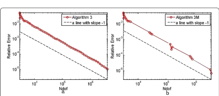
Algorithm 3M, respectively. The results are shown in Tables 1–3. We depict the error curves of Algorithms 1–3 and Algorithms 1M–3M in Figs. 1–3.
From Tables 1–3, we can get the conclusion that in the case the accurate are almost same, Algorithms 2–3 take about half time of Algorithm 1. In the case the accurate are almost same, AlgorithmiM takes about25time of Algorithmi,i= 1, 2, 3.
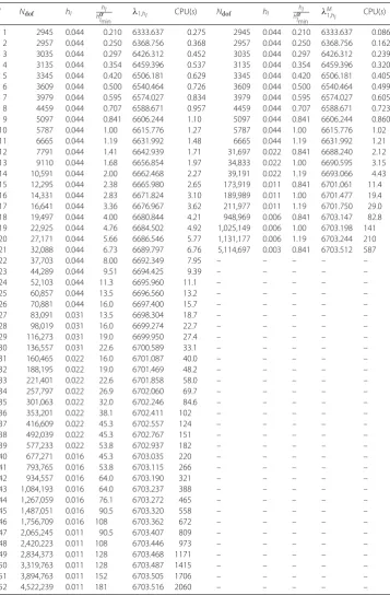
Table 1 The smallest eigenvalue solved by Algorithm 1 and Algorithm 1M
l Ndof hl hαhl
lmin
λ1,hl CPU(s) Ndof hl hαhl
lmin λM
1,hl CPU(s)
1 2945 0.044 0.210 6333.637 0.275 2945 0.044 0.210 6333.637 0.086
2 2957 0.044 0.250 6368.756 0.368 2957 0.044 0.250 6368.756 0.162
3 3035 0.044 0.297 6426.312 0.452 3035 0.044 0.297 6426.312 0.239
4 3135 0.044 0.354 6459.396 0.537 3135 0.044 0.354 6459.396 0.320
5 3345 0.044 0.420 6506.181 0.629 3345 0.044 0.420 6506.181 0.405
6 3609 0.044 0.500 6540.464 0.726 3609 0.044 0.500 6540.464 0.499
7 3979 0.044 0.595 6574.027 0.834 3979 0.044 0.595 6574.027 0.605
8 4459 0.044 0.707 6588.671 0.957 4459 0.044 0.707 6588.671 0.723
9 5097 0.044 0.841 6606.244 1.10 5097 0.044 0.841 6606.244 0.860
10 5787 0.044 1.00 6615.776 1.27 5787 0.044 1.00 6615.776 1.02
11 6665 0.044 1.19 6631.992 1.48 6665 0.044 1.19 6631.992 1.21
12 7791 0.044 1.41 6642.939 1.71 31,697 0.022 0.841 6688.240 2.12
13 9110 0.044 1.68 6656.854 1.97 34,833 0.022 1.00 6690.595 3.15
14 10,591 0.044 2.00 6662.468 2.27 39,191 0.022 1.19 6693.066 4.43
15 12,295 0.044 2.38 6665.980 2.65 173,919 0.011 0.841 6701.061 11.4
16 14,331 0.044 2.83 6671.824 3.10 189,989 0.011 1.00 6701.477 19.4
17 16,641 0.044 3.36 6676.967 3.62 211,977 0.011 1.19 6701.750 29.0
18 19,497 0.044 4.00 6680.844 4.21 948,969 0.006 0.841 6703.147 82.8
19 22,925 0.044 4.76 6684.502 4.92 1,025,149 0.006 1.00 6703.198 141 20 27,171 0.044 5.66 6686.546 5.77 1,131,177 0.006 1.19 6703.244 210 21 32,088 0.044 6.73 6689.797 6.76 5,114,697 0.003 0.841 6703.512 587
22 37,703 0.044 8.00 6692.349 7.95 – – – – –
23 44,289 0.044 9.51 6694.425 9.39 – – – – –
24 52,103 0.044 11.3 6695.960 11.1 – – – – –
25 60,857 0.044 13.5 6696.560 13.2 – – – – –
26 70,881 0.044 16.0 6697.400 15.7 – – – – –
27 83,091 0.031 13.5 6698.304 18.7 – – – – –
28 98,019 0.031 16.0 6699.274 22.7 – – – – –
29 116,273 0.031 19.0 6699.950 27.4 – – – – –
30 136,557 0.031 22.6 6700.589 33.1 – – – – –
31 160,465 0.022 16.0 6701.087 40.0 – – – – –
32 188,195 0.022 19.0 6701.469 48.2 – – – – –
33 221,401 0.022 22.6 6701.858 58.0 – – – – –
34 257,797 0.022 26.9 6702.060 69.7 – – – – –
35 301,063 0.022 32.0 6702.246 84.6 – – – – –
36 353,201 0.022 38.1 6702.411 102 – – – – –
37 416,609 0.022 45.3 6702.557 124 – – – – –
38 492,039 0.022 45.3 6702.767 151 – – – – –
39 577,233 0.022 53.8 6702.937 182 – – – – –
40 677,271 0.016 45.3 6703.035 220 – – – – –
41 793,765 0.016 53.8 6703.115 266 – – – – –
42 934,557 0.016 64.0 6703.190 321 – – – – –
43 1,084,193 0.016 64.0 6703.237 388 – – – – –
44 1,267,059 0.016 76.1 6703.272 465 – – – – –
45 1,487,051 0.016 90.5 6703.320 558 – – – – –
46 1,756,709 0.016 108 6703.362 672 – – – – –
47 2,065,245 0.011 90.5 6703.407 809 – – – – –
48 2,420,223 0.011 108 6703.446 973 – – – – –
49 2,834,373 0.011 128 6703.468 1171 – – – – –
50 3,319,763 0.011 128 6703.487 1415 – – – – –
51 3,894,763 0.011 152 6703.505 1706 – – – – –
52 4,522,239 0.011 181 6703.516 2060 – – – – –
InR3, the initial meshπ
h0is tetrahedron subdivision with mesh size
√ 3
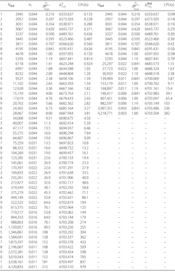
Table 2 The smallest eigenvalue solved by Algorithm 2 and Algorithm 2M
l Ndof hl hαhl
lmin λR
1,hl CPU(s) Ndof hl hαhl
lmin λRM
1,hl CPU(s)
1 2945 0.044 0.210 6333.637 0.133 2945 0.044 0.210 6333.637 0.090
2 2957 0.044 0.297 6373.503 0.228 2957 0.044 0.297 6373.503 0.140
3 3031 0.044 0.354 6538.971 0.280 3031 0.044 0.354 6538.971 0.192
4 3067 0.044 0.420 6443.737 0.371 3067 0.044 0.420 6443.737 0.250
5 3237 0.044 0.500 6489.761 0.426 3237 0.044 0.500 6489.761 0.305
6 3445 0.044 0.595 6523.466 0.487 3445 0.044 0.595 6523.466 0.365
7 3811 0.044 0.707 6566.620 0.560 3811 0.044 0.707 6566.620 0.431
8 4195 0.044 0.841 6595.431 0.636 4195 0.044 0.841 6595.431 0.504
9 4678 0.044 1.00 6597.955 0.720 4678 0.044 1.00 6597.955 0.588
10 5293 0.044 1.19 6607.441 0.814 5293 0.044 1.19 6607.441 0.709
11 6118 0.044 1.41 6623.248 0.924 25,297 0.022 0.841 6683.573 1.15
12 6997 0.044 1.68 6634.588 1.05 27,723 0.022 1.00 6686.324 1.63
13 8232 0.044 2.00 6648.804 1.20 30,933 0.022 1.19 6688.518 2.38
14 9527 0.044 2.38 6658.106 1.39 139,409 0.011 0.841 6700.069 5.87
15 11,102 0.044 2.83 6663.393 1.59 153,179 0.011 1.00 6700.762 9.71
16 12,928 0.044 3.36 6667.166 1.82 168,897 0.011 1.19 6701.161 15.4
17 15,139 0.044 4.00 6673.763 2.11 740,417 0.006 0.841 6702.983 39.1
18 17,619 0.044 4.76 6678.433 2.43 807,451 0.006 1.00 6703.097 65.4
19 20,763 0.044 5.66 6682.562 2.82 882,597 0.006 1.19 6703.149 103
20 24,365 0.044 6.73 6685.164 3.27 3,907,351 0.003 0.841 6703.486 236 21 28,967 0.044 8.00 6687.944 3.81 4,218,771 0.003 1.00 6703.504 382
22 34,068 0.044 9.51 6690.675 4.50 – – – – –
23 40,007 0.044 11.3 6692.914 5.39 – – – – –
24 47,117 0.044 13.5 6694.937 6.46 – – – – –
25 55,275 0.044 16.0 6696.294 7.64 – – – – –
26 64,407 0.044 19.0 6696.867 9.09 – – – – –
27 75,259 0.031 13.5 6697.823 10.8 – – – – –
28 88,353 0.031 16.0 6698.752 13.2 – – – – –
29 104,269 0.031 19.0 6699.457 16.1 – – – – –
30 123,285 0.031 22.6 6700.133 19.4 – – – – –
31 145,061 0.031 26.9 6700.774 23.3 – – – – –
32 170,397 0.022 22.6 6701.291 27.9 – – – – –
33 199,833 0.022 26.9 6701.638 33.5 – – – – –
34 235,261 0.022 26.9 6701.906 40.0 – – – – –
35 272,877 0.022 32.0 6702.117 48.6 – – – – –
36 319,549 0.022 38.1 6702.292 58.8 – – – – –
37 375,279 0.022 45.3 6702.462 71.1 – – – – –
38 444,149 0.022 53.8 6702.631 86.1 – – – – –
39 522,525 0.022 64.0 6702.819 104 – – – – –
40 613,375 0.022 76.1 6702.964 125 – – – – –
41 719,217 0.016 53.8 6703.062 149 – – – – –
42 844,333 0.016 64.0 6703.144 179 – – – – –
43 988,863 0.016 76.1 6703.208 214 – – – – –
44 1,150,057 0.016 90.5 6703.256 255 – – – – –
45 1,346,861 0.016 108 6703.292 304 – – – – –
46 1,584,041 0.016 128 6703.337 362 – – – – –
47 1,873,597 0.016 152 6703.378 433 – – – – –
48 2,196,067 0.011 108 6703.422 509 – – – – –
49 2,572,281 0.011 128 6703.454 598 – – – – –
50 3,010,543 0.011 152 6703.474 705 – – – – –
51 3,538,161 0.011 181 6703.497 831 – – – – –
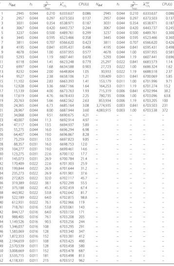
Table 3 The smallest eigenvalue solved by Algorithm 3 and Algorithm 3M
l Ndof hl hαhl
lmin λF
1,hl CPU(s) Ndof hl hαhl
lmin λFM
1,hl CPU(s)
1 2945 0.044 0.210 6333.637 0.086 2945 0.044 0.210 6333.637 0.086
2 2957 0.044 0.297 6373.503 0.137 2957 0.044 0.297 6373.503 0.137
3 3031 0.044 0.354 6538.971 0.187 3031 0.044 0.354 6538.971 0.187
4 3067 0.044 0.420 6443.737 0.244 3067 0.044 0.420 6443.737 0.245
5 3237 0.044 0.500 6489.761 0.299 3237 0.044 0.500 6489.761 0.300
6 3445 0.044 0.595 6523.466 0.358 3445 0.044 0.595 6523.466 0.360
7 3811 0.044 0.707 6566.620 0.423 3811 0.044 0.707 6566.620 0.426
8 4195 0.044 0.841 6595.431 0.496 4195 0.044 0.841 6595.431 0.498
9 4678 0.044 1.00 6597.955 0.577 4678 0.044 1.00 6597.955 0.581
10 5293 0.044 1.19 6607.441 0.670 5293 0.044 1.19 6607.441 0.696
11 6118 0.044 1.41 6623.248 0.779 25,297 0.022 0.841 6683.573 1.14
12 6997 0.044 1.68 6634.588 0.903 27,723 0.022 1.00 6686.324 1.62
13 8232 0.044 2.00 6648.804 1.05 30,933 0.022 1.19 6688.518 2.37
14 9527 0.044 2.38 6658.106 1.21 139,409 0.011 0.841 6700.069 5.85
15 11,102 0.044 2.83 6663.393 1.41 153,179 0.011 1.00 6701.996 9.71
16 12,928 0.044 3.36 6667.166 1.64 164,253 0.011 1.19 6701.274 15.2
17 15,139 0.044 4.00 6673.763 1.93 715,319 0.006 0.841 6702.994 38.2
18 17,619 0.044 4.76 6678.433 2.25 780,735 0.006 1.00 6703.096 63.8
19 20,763 0.044 5.66 6682.562 2.63 853,934 0.006 1.19 6703.205 100
20 24,365 0.044 6.73 6685.164 3.08 3,774,935 0.003 0.841 6703.503 231 21 28,967 0.044 8.00 6687.944 3.60 4,083,915 0.003 1.00 6703.538 372
22 34,068 0.044 9.51 6690.675 4.21 – – – – –
23 40,007 0.044 11.3 6692.914 4.97 – – – – –
24 47,117 0.044 13.5 6694.937 5.89 – – – – –
25 55,275 0.044 16.0 6696.294 6.98 – – – – –
26 64,407 0.044 19.0 6696.867 8.28 – – – – –
27 75,259 0.031 13.5 6697.823 9.85 – – – – –
28 88,357 0.031 16.0 6698.753 12.0 – – – – –
29 104,277 0.031 19.0 6699.461 14.6 – – – – –
30 123,275 0.031 22.6 6700.132 17.7 – – – – –
31 145,073 0.031 26.9 6700.784 21.4 – – – – –
32 170,409 0.022 22.6 6701.303 25.9 – – – – –
33 199,844 0.022 26.9 6701.644 31.2 – – – – –
34 235,273 0.022 26.9 6701.901 37.6 – – – – –
35 272,825 0.022 32.0 6702.117 45.7 – – – – –
36 319,389 0.022 38.1 6702.299 55.5 – – – – –
37 375,188 0.022 45.3 6702.459 67.4 – – – – –
38 443,902 0.022 53.8 6702.642 81.7 – – – – –
39 522,189 0.022 64.0 6702.815 98.8 – – – – –
40 612,931 0.022 76.1 6702.966 119 – – – – –
41 718,761 0.016 53.8 6703.061 143 – – – – –
42 844,127 0.016 64.0 6703.150 171 – – – – –
43 988,405 0.016 76.1 6703.208 205 – – – – –
44 1,149,526 0.016 90.5 6703.256 244 – – – – –
45 1,346,037 0.016 108 6703.295 291 – – – – –
46 1,583,069 0.016 128 6703.340 347 – – – – –
47 1,872,353 0.016 152 6703.381 412 – – – – –
48 2,194,659 0.011 108 6703.425 490 – – – – –
49 2,570,539 0.011 128 6703.458 580 – – – – –
50 3,008,669 0.011 152 6703.478 687 – – – – –
51 3,535,715 0.011 181 6703.498 813 – – – – –
Figure 1The convergence rates of the smallest eigenvalue from Algorithm 1(a) and Algorithm 1M(b)
Figure 2The convergence rates of the smallest eigenvalue from Algorithm 2(a) and Algorithm 2M(b)
[image:19.595.117.477.456.614.2]Figure 4The refined mesh for the L-shaped domain (a) and the convergence rates of the smallest eigenvalue from Algorithm 1 and Algorithm 2(b) inR3
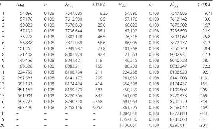
Table 4 The smallest eigenvalue solved by Algorithm 1 and Algorithm 2
l Ndof hl λ1,hl CPU(s) Ndof hl λR1,hl CPU(s)
1 54,896 0.108 7547.686 8.25 54,896 0.108 7547.686 9.71
2 57,176 0.108 7612.980 16.5 57,176 0.108 7613.142 13.0
3 60,822 0.108 7678.863 25.6 60,822 0.108 7678.902 16.7
4 67,192 0.108 7736.644 35.1 67,192 0.108 7736.699 20.9
5 76,278 0.108 7802.128 46.5 76,316 0.108 7802.062 25.8
6 86,838 0.108 7871.038 58.6 86,905 0.108 7872.137 31.2
7 101,261 0.108 7949.987 73.8 101,368 0.108 7950.349 38.4
8 121,408 0.108 8001.974 92.4 121,563 0.108 8002.931 47.3
9 146,456 0.108 8041.421 118 146,215 0.108 8040.738 58.1
10 180,528 0.108 8082.211 155 180,203 0.108 8082.247 72.3
11 224,755 0.108 8108.734 211 224,288 0.108 8108.530 92.1
12 282,583 0.108 8141.177 295 281,953 0.108 8141.009 119
13 355,133 0.108 8174.424 414 354,598 0.108 8174.437 156
14 451,162 0.108 8199.573 583 450,739 0.108 8199.502 205
15 561,904 0.108 8220.566 847 561,090 0.108 8220.433 269
16 693,222 0.108 8240.310 2368 691,963 0.108 8240.129 354
17 863,420 0.108 8258.156 9957 861,795 0.108 8258.042 469
18 – – – – 1,084,848 0.108 8272.888 624
19 – – – – 1,357,830 0.108 8281.060 851
20 – – – – 1,730,050 0.108 8290.011 1206
BecauseNdofinR3increases very fast after uniform refinement, which leads to surpassing computer’s memory, we cannot employ Algorithms 1M–3M to solve (2.1).
Acknowledgements
This work is supported by the Science and Technology Foundation of Guizhou Province of China (Grant nos. LH [2014] 7061 and LKS [2013] 06). We appreciate editors and reviewers for constructive suggestions and helpful comments.
Competing interests
The authors declare to have no competing interests.
Authors’ contributions
HL and YY participated in the theoretical analysis and HL carried out the numerical experiments. The final manuscript was made after YY had discussed it with HL. All authors read and approved the final manuscript.
Publisher’s Note
[image:20.595.118.478.314.534.2]Received: 8 December 2017 Accepted: 20 February 2018 References
1. Morley, L.S.D.: The triangular equilibrium element in the solution of plate bending problems. Aero Quart (1968) 2. Wang, M., Xu, J.: The Morley element for fourth order elliptic equations in any dimensions 155-169. Numer. Math.103,
155–169 (2006)
3. da Veiga, L.B., Niiranen, J., Stenberg, R.: A posteriori errors estimates for the Morley plate bending element. Numer. Math.106, 165–179 (2007)
4. Hu, J., Shi, Z.: A new a posteriori error estimate for the Morley element. Numer. Math.112, 25–40 (2009) 5. Shi, Z., Wang, M.: Finite Element Methods. Science Press, Beijing (2013)
6. Carstensen, C., Gallistl, D., Hu, J.: A posteriori error estimates for nonconforming finite element methods for fourth-order problems on rectangles. Numer. Math.124, 309–335 (2013)
7. Hu, J., Shi, Z., Xu, J.: Convergence and optimality of the adaptive Morley method. Numer. Math.121, 731–752 (2012) 8. Carstensen, C., Gallistl, D., Hu, J.: A discrete Helmholtz decomposition with Morley finite element functions and the
optimality of adaptive finite element schemes. Comput. Math. Appl.68(part B), 2167–2181 (2014)
9. Rannacher, R.: Nonconforming finite element methods for eigenvalue problems in linear plate theory. Numer. Math.
13, 23–42 (1979)
10. Shen, Q.: A posteriori error estimates of the Morley element for the fourth order elliptic eigenvalue problem. Numer. Algorithms68, 455–466 (2015)
11. Yang, Y., Li, H., Bi, H.: The lower bound property of the Morley element eigenvalues. Comput. Math. Appl.17, 904–920 (2016)
12. Gallistl, D.: Morley finite element method for the eigenvalues of the biharmonic operator. IMA J. Numer. Anal.35(4), 1779–1811 (2015)
13. Babuška, I., Rheinboldt, W.C.: Error estimates for adaptive finite element computations. SIAM J. Numer. Anal.15, 736–754 (1978)
14. Verfürth, R.: A Review of a Posteriori Error Estimates and Adaptive Mesh-Refinement Techniques. Wiley-Teubner, New York (1996)
15. Ainsworth, M., Oden, J.T.: A Posteriori Error Estimates in the Finite Element Analysis. Wiley-Inter science, New York (2011)
16. Morin, P., Nochetto, R.H., Siebert, K.: Convergence of adaptive finite element methods. SIAM Rev.44, 631–658 (2002) 17. Yang, Y., Bi, H., Han, J., Yu, Y.: The shifted-inverse iteration based on the multigrid discretizations for eigenvalue
problems. SIAM J. Sci. Comput.37, 2583–2606 (2015)
18. Blum, H., Rannacher, R.: On the boundary value problem of the biharmonic operator on domains with angular corners. Math. Methods Appl. Sci.2, 556–581 (1980)
19. Li, H., Yang, Y.:c0ipg adaptive algorithms for the biharmonic eigenvalue problem. Numer. Algorithms (2017). https://doi.org/10.1007/s11075-017-0388-8
20. Ciarlet, P.G.: Basic Error Estimates for Elliptic Problems. Handbook of Numerical Analysis, vol. 2. Elsevier, North-Holand (1991)
21. Babuška, I., Kellog, R.B., Pitkaranta, J.: Direct and inverse error estimates for finite elements with mesh refinement. Numer. Math.33, 447–471 (1979)
22. Hu, J., Huang, Y., Lin, Q.: Lower bounds for eigenvalues of elliptic operators: by nonconforming finite element methods. J. Sci. Comput.61, 196–221 (2014)
23. Lin, Q., Xie, H., Xu, J.: Lower bounds of the discretization for piecewise polynomials. Math. Comput.83, 1–13 (2014) 24. Carstensen, C., Gallistl, D.: Guaranteed lower eigenvalue bounds for the biharmonic equation. Numer. Math.125,
33–51 (2014)
25. Yang, Y., Zhang, Z., Lin, F.: Eigenvalue approximation from below using nonforming finite elements. Sci. China Math.
53, 137–150 (2010)
26. Yang, Y., Bi, H.: A tow-grid discretization scheme based on shifted-inverse power method. SIAM J. Numer. Anal.49, 1602–1642 (2011)
27. Dai, X., Xu, J., Zhou, A.: Convergence and optimal complexity of adaptive finite element eigenvalue computations. Numer. Math.110, 313–355 (2008)