Multivariate complexity analysis of 3D surface form and function of centric diatoms at the Eocene–Oligocene transition

Multivariate complexity analysis of 3D surface form and function of

centric diatoms at the Eocene

–

Oligocene transition

Janice L. Pappas

Museum of Paleontology, University of Michigan, 1109 Geddes Avenue, Ann Arbor, MI 48109-1079, USA

a b s t r a c t

a r t i c l e i n f o

Article history: Received 19 June 2015

Received in revised form 7 December 2015 Accepted 12 December 2015

Available online 17 December 2015

Complexity is important in the course of evolution, but consensus of what complexity analysis entails is elusive. In this study, multivariate complexity is measured and analyzed in terms of magnitude of change and the trends behind those changes. Multivariate morphological and functional complexities were analyzed using 3D surface models of centric diatom genera from the Eocene to Oligocene, a transitional time when temperatures cooled, sea levels rose, and glaciation increased. Diatoms were chosen for study because of their importance in biostra-tigraphy, biogeochemical cycling, productivity, food web dynamics, and sensitivity to environmental conditions.

Probabilistic analysis using a Markov chain indicated an increase in total complexity across the Eocene–Oligocene

transition (EOT). Causal inference via structural equation modeling indicated weakly driven functional and mor-phological complexity trends over the EOT. Mormor-phological and functional complexity trends differed with respect to predation resistance as responses to ecological complexity as environmental and climate change occurred across the EOT. Macroevolutionary patterns of morphological and functional complexity with respect to ecolog-ical complexity did not necessarily coincide over time.

© 2015 Elsevier B.V. All rights reserved. Keywords:

Diatoms 3D morphology Jacobian

Morphological complexity Functional complexity Predation resistance Macroevolution

1. Introduction

That organisms become more complex over time has been espoused as the dominant viewpoint in biology (e.g.,Lamarck, 1809; Darwin, 1859; Miconi, 2008; McShea and Brandon, 2010; Auerbach and Bongard, 2014) because evolution has occurred from unicellular to mul-ticellular entities. The nominal basis for this claim is that by counting cells, complexity can be determined (e.g.,Wicken, 1979; McShea, 1991; McShea and Brandon, 2010). Aside from this obvious pronounce-ment, no consensus exists on the definition of complexity (especially over multiple disciplines), analyses have entailed discordant ap-proaches, and equivocal results have been produced (McNamara, 2006). Complexity of organisms has been based on various attributes such as size (e.g.,McShea and Brandon, 2010; McShea and Hordijk, 2013), body plan (Valentine, 2000), heterogeneity or degree of differentiation (Darwin, 1859), and pattern arrangement of number of parts (e.g.,McShea, 1991, 1992; McShea and Venit, 2001). Complexity is usu-ally determined at a one- (1D) or two-dimensional scale (2D) or level (e.g.,McShea, 1991; McShea and Brandon, 2010) where, e.g., bits of in-formation and their sequential structure are assessed (e.g.,McShea, 1992; Adami, 2002). Whenever questions arise about the definition of complexity or parts, qualifiers (e.g.,McShea and Venit, 2001), nuanced descriptions (e.g.,McShea, 1992; McShea and Brandon, 2010), or nega-tion terms (e.g.,Wicken, 1979; McShea, 1991) are invoked in order to

legitimize the methods used in complexity analysis. Definitions of parts and whole entities with respect to complexity are described, which are dependent on boundary determinations, which in turn are context and scale dependent and must be defined a priori for complex-ity analysis to begin. Applying such constraints across the board pre-sents difficulties in generalizing complexity measurement and analysis and arriving at a consensus on what is meant by complexity.

At the other end of the spectrum, complex systems are analyzed by treating different organisms as“particles”and applying a particular al-gorithm such as an artificial neural network via agent-based modeling (e.g.,Yaeger et al., 2008) to determine large scale complexity trends. While results have been intriguing (e.g., Auerbach and Bongard, 2014), computational complexity sometimes substitutes for biological complexity (e.g.,Adami, 2002), and meaningful attributes of actual or-ganisms and their significance are not necessarily recovered by such methods. In spite of this, many 1D and 2D systems-based assessments express complexity change over time as probabilistic (e.g.,Yaeger et al., 2008; McShea and Brandon, 2010). By using a probability-based framework, the likelihood of a future event of complexity change and its trend over time can be inferred as a result rather than merely counting and cataloging the frequency of past events of complexity change. To start, measuring complexity as a deterministic quantity aids in circumventing the need for elaborate, specific descriptions and conceptualizations in order to constrain analyses tofit the purposes of isolated studies.

Complexity as a deterministic quantity is useful in studying a single event or determining a long term macroevolutionary trend where

E-mail address:[email protected].

http://dx.doi.org/10.1016/j.marmicro.2015.12.001 0377-8398/© 2015 Elsevier B.V. All rights reserved.

Contents lists available atScienceDirect

Marine Micropaleontology

form is important in the evolution and coevolution of organisms. Differ-ent types of complexity as deterministic quantities can be aggregated as

n-dimensional measures. Complexity as a multidimensional quantity enables its assessment asn-macroevolutionary trends, with potentially different magnitudes and/or drivers for each trend. Understanding the differences may enable discernment of long term patterns of complexity changes in evolution.

1.1. Purposes of the study

Multicellular taxa are typically chosen for study in complexity analysis (e.g.,McShea, 1992), since it is taken for granted that only multicellular organisms qualify. However, complexity assessment is a comparative exercise, and among the unicells, diatoms possess complex morphology (Harwood et al., 2007), representing a mono-phyletic group at the class or phylum level (Williams and Kociolek, 2007). Diatoms account for at least 40% of total productivity, 50% of or-ganic carbon sequestration in the sediment (Falkowski et al., 2004), and are important in the global carbon (Hopkinson et al., 2011) and silica (Knoll, 2003) cycles. Diatoms are biogeochemically and stratigraphically important in characterizing paleoenvironments and paleoclimates as a re-sult of their ubiquitous distribution and diversity (e.g.,Harwood et al., 2007; Jordan and Stickley, 2010). Upwelling affected silica cycling and productivity in surface waters throughout the Cenozoic, and since the Ol-igocene, diatoms are the dominant contributors to the global silica cycle as evidenced by their high sedimentation rate (Harwood et al., 2007; Witkowski et al., 2014). Limiting conditions for silica availabil-ity (Conley, 2002; Harwood et al., 2007) and other nutrients in the oceans control not only diatom productivity, evolution and diversifi -cation (Jordan and Stickley, 2010), but also diatom morphological features and the degree to which they are silicified (Barron and Baldauf, 1989).

The Eocene–Oligocene transition (EOT) is an important period of changing composition of diatom taxa during the Cenozoic (Jordan and Stickley, 2010) because of changes from increasing levels of atmospher-ic CO2with greenhouse temperatures and high sea levels during the Eo-cene to low levels of atmospheric CO2, with icehouse temperatures and low sea levels with ice sheet expansion in the Oligocene (Zachos et al., 2008; Jordan and Stickley, 2010). Centric diatoms contributed to a major shift in global carbon cycling and increasing oxygenation of sur-face waters during the change from greenhouse to icehouse conditions (Armbrust, 2009). Since the Cretaceous, centric diatoms have endured, survived and proliferated, exhibiting a wide variety of morphologies (Harwood et al., 2007). Although centric diatoms were prevalent during the Cenozoic, morphological and functional complexity are neither eas-ily discernible upon cursory inspection of the taxa nor is the relation be-tween complexity and environmental and climate conditions evident during this time.

To measure complexity in centric diatoms from the Eocene and Oli-gocene, three-dimensional (3D) surface models will be devised using parametric 3D equations (Pappas, 2005a, 2005b, 2008; Pappas and Miller, 2013), and their numerical solution will be used in measurement of morphological complexity. Functional complexity will be measured as a quantity with respect to surface area extracted from measurement of morphological complexity. Morphological and functional complexity will be aggregated as multivariate quantities, and from this, rank order-ing of taxa from the Eocene to the Oligocene will serve as a vector of complexity change over time. Magnitude of short and long term com-plexity change will be probabilistically analyzed and measured with re-gard to steady-state conditions. Causal inference will be used to determine mode of complexity as an evolutionary trend using multivar-iate modeling and probabilistic analysis. The context of morphological and functional complexity will be examined in terms of ecological changes that occurred during the EOT.

Measuring complexity is not the same as measuring diversity. Com-plexity is not about counting the number of all the different taxa that existed in the Eocene and Oligocene. To attempt to consider every last possible taxon, especially rare or accidental occurrences, is neither at-tainable nor necessary. Rather, complexity is about the number of differ-ent kinds of surface morphological patterns common among taxa. Surface morphological patterns are redundant over a number of differ-ent taxa (e.g.,Barber and Haworth, 1981), and for a circumscribed time period from the Eocene to the Oligocene, afinite number of pat-terns occur. Such patpat-terns fall into succinct categories based on surface geometry.

Geometrically, whole diatom frustules are capped cylinders. On their exterior valve faces, layers of pores or foramina are arranged in various patterns (Round et al., 1990). Areolae or puncta can be spaced regularly or irregularly, change in size or shape, be radiating from one spot, ar-ranged concentrically from the center, or lined up in a parallel fashion (Barber and Haworth, 1981). Rows of areolae or puncta may form a dis-continuous, random, sparse, or dense pattern (Barber and Haworth, 1981). In spite of the vast array of possible combinations of features on their frustule surfaces, redundant centric diatom structural geomet-ric features are commonly recognized over many taxa.

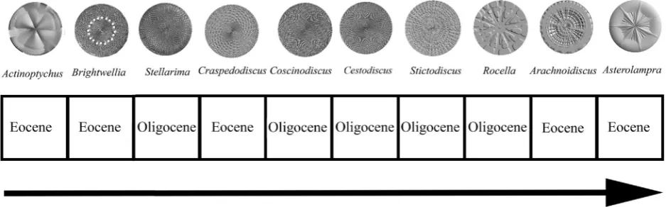
These surface morphological patterns are discernable from taxa in the Eocene and Oligocene, where diatoms are indicative of the prevail-ing environmental and climate conditions and are accumulated in the sediments via rapid burial or from lack of exposure to high alkalinity and high temperature pore waters (e.g.,Barron and Baldauf, 1989, 1995). For selection purposes, taxa may be grouped by traditional mor-phological classification categories since a monophyletic tree of diatom taxa has yet to be realized (e.g.,Williams and Kociolek, 2007; Theriot et al., 2010, 2011). Classification groups specified inFenner (1985) andRound et al. (1990)are used as general non-phylogenetic taxonom-ic bins although these descriptors have been used in phylogenettaxonom-ic as-sessments (e.g.,Williams and Kociolek, 2007; Theriot et al., 2010, 2011). Taxon groups in the Coscinodiscophyceae (e.g.,Round et al., 1990; Williams and Kociolek, 2007) characterize many of the centric taxa from the Eocene and Oligocene consisting of the Coscinodiscales, Stictodiscales, Arachnoidiscales, and Asterolamprales (e.g.,Fenner, 1985; Round et al., 1990). Of these taxon orders, particular gross geom-etries on the valve face can be described in terms of different sizes and degrees of pores and distinct arrangements of surface features in a radi-ating pattern (e.g.,Barber and Haworth, 1981; Round et al., 1990). From actual centric taxa obtained from Eocene and Oligocene sediments, pub-lished accounts from the Deep Sea Drilling Project (DSDP), Ocean Dril-ling Program (ODP), Integrated Ocean DrilDril-ling Program (IODP), and the United States Geological Survey (USGS) are used to determine the pool of taxa from which to select exemplars of surface geometry having the specific arrangement of pores or radiating features mentioned above. As a result, diatom biostratigraphic markers qualify as the best means to select exemplars of surface morphological patterns for com-plexity analysis.

The particular centric diatom genera that were chosen from which to make 3D surface models have been restricted to those in the Coscinodiscophyceae with an approximate circular valve and cross-sectional shape and cylindrical 3D shape. This will enable the elimina-tion of overall shape as a confounding factor and make modeling of the taxa for comparative purposes simpler. Taxon selection representing surface morphology was based on specific criteria: (1) the importance of the taxon in diatom biostratigraphy; (2) relative abundance for a given time period; and/or (3) whether a species from a genus was a marker atfirst or last occurrence. These taxa may have originated at an earlier time or occur in both the Eocene and Oligocene, but many published reports were used to obtain the best consensus of information from which to choose centric diatom genera. Diatom zona-tion is an ongoing refinement process governed byfirst and last taxon appearances, reconciling different zonation schemes, incomplete strati-graphic sequences, and matching diatom to calcareous nanofossil zones (e.g.,Barron and Baldauf, 1989) or magnetostratigraphy (e.g.,Barron and Baldauf, 1995). Opal deposition at different latitudes, regions and oceans, and non-continuous cores of diatom-containing sediments are considerations for matching diatom zones, and dissolution, bioturba-tion, or diagenesis introducing biases in discerning the fossil diatom re-cord (e.g.,Harwood et al., 2007) further complicate the matching of different zonation schemes. However, there is much agreement in dia-tom zone correlations so that particular centric diadia-tom genera can be construed to be representative or important in either the Eocene or Ol-igocene for the purposes of this study. For the entire formal probability selection process, see theAppendix A.

The Eocene–Oligocene centric diatom genera are assembled from published accounts inHajόs (1976),Gombos (1983a, 1983b, 1987), Gombos and Ciesielski (1983),Fenner (1984a, 1984b, 1985),Barron (1985),Baldauf and Barron (1987),Saito et al. (1988),Baldauf and Monjanel (1989),Fenner and Mikkelsen (1990),Fourtanier (1991), Harwood and Maruyama (1992),Barron and Mahood (1993),Barron and Baldauf (1995),Arney et al. (2003),Barron et al. (2004),Bohaty et al. (2011),Oreshkina (2012), andGladenkov (2012).

Representative genera chosen as the basis for 3D surfaces models are:ActinoptychusC. G. Ehrenberg, typically found in the Early to Middle Eocene (Fenner, 1985);ArachnoidiscusDeane ex Pritchard, which is considered to be robust to preservation issues (Fenner and Mikkelsen, 1990) and a representative of the Early Eocene (Fourtanier, 1991);

Asterolampra C. G. Ehrenberg, where Asterolampra marylandica

Ehrenberg is representative of the Middle to earliest Late Eocene (Fenner, 1984a, 1984b, 1985; Fenner and Mikkelsen, 1990; Barron and Baldauf, 1995) and the genus is prevalent (Fenner, 1985);Brightwellia

J. Ralfs in A. Pritchard, whereBrightwellia hyperboreaGrunow is repre-sentative of the Middle Eocene (Gombos, 1983b; Fenner, 1985; Barron and Baldauf, 1995; Oreshkina, 2012);CraspedodiscusC. G. Ehrenberg, whereCraspedodiscus oblongus(Greville) Grunow in A. Schmidt is rep-resentative of the Early Eocene (Fenner, 1985; Fourtanier, 1991; Barron and Baldauf, 1995).

Genera chosen for study representing the Oligocene are:Cestodiscus

Greville, whereCestodiscus reticulatusFenner is important in the Early Oligocene (Fenner, 1985; Barron and Baldauf, 1995; Barron et al., 2004), with 50 to 80% of diatom assemblages being composed of

Cestodiscusspecies;CoscinodiscusC. G. Ehrenberg, whereCoscinodiscus excavatusGreville is important in the Early Oligocene (Fenner, 1985; Barron and Baldauf, 1995; Barron et al., 2004) and many other species are present throughout the Oligocene (Barron and Mahood, 1993);

RocellaHanna, whereRocella vigilansFenner (Oligocene) andRocella gelida(Mann) Bukry (Oligocene into the Miocene) (Gombos and Ciesielski, 1983; Fenner, 1984a, 1984b, 1985; Baldauf and Barron, 1987; Baldauf and Monjanel, 1989; Barron and Baldauf, 1995) are im-portant. Two additional genera are chosen to be used as Oligocene rep-resentatives based on relative abundances even though these taxa may have originated in the Upper Cretaceous (Harwood and Nikolaev, 1995). The genera are:StellarimaHasle and Sims, the species of which

occur frequently (Baldauf and Barron, 1987; Saito et al., 1988), with the genus containing long-ranging taxa (Scherer et al., 2000; Witkowski and Harwood, 2011);StictodiscusR. K. Greville, where spe-cies are common,Stictodiscus kittonianusGreville is a key marker species (Baldauf and Barron, 1987; Barron and Mahood, 1993; Arney et al., 2003), with the genus containing long-ranging taxa (Scherer et al., 2000). Actinoptychus,Arachnoidiscus, and Stictodiscus are benthic,

Actinoptychusalso has some planktonic species, and all other taxa are planktonic (Baldauf and Barron, 1987). All taxon names were checked using the following: G Dallas Hanna Database (Catalog of Diatom Names, California Academy of Sciences, On-line Version updated 19 Sep. 2011. Compiled by Elisabeth Fourtanier and J. Patrick Kociolek. Available online athttp://research.calacademy.org/research/diatoms/ names/index.asp); ITIS (http://www.itis.gov); WoRMS (http://www. marinespecies.org).

Diatom specimens are not well preserved over long periods of geo-logic time (Barron and Baldauf, 1995; Harwood et al., 2007), because opaline silica will dissolve in alkaline waters and warm temperatures where the longer the diatom is exposed to seawater, the more likely it is to dissolve. Opal deposition is subject to diagenesis (Barron and Baldauf, 1995) and will accumulate in upwelling regions where there has been high productivity (Fenner, 1985). Using a 3D surface modeling technique enables control of the quantity (large numbers of specimens can be made), quality (no taphonomic alterations), andfidelity (models capturing essential geometric characteristic features of morphology) of model specimens. Time and expense of acquiring the appropriate spec-imens for study is also minimized. Published micrographs on diatom taxa are readily available via the Internet on which to base 3D surface morphology models. Diatom biomechanical data is scant, and using 3D surface models to extrapolate values in concert with empirical data enables functional complexity analysis.

The 3D surface morphologies for each diatom genus are constructed as hybrid surface patterns based on light and/or scanning electron mi-crographs of taxa as pictured in the following: Hajόs (1976) (Arachnoidiscus Coscinodiscus), Gombos (1983a) (Asterolampra,

Brightwellia,Stellarima),Gombos and Ciesielski (1983)(Asterolampra,

Brightwellia, Coscinodiscus, Rocella, Stictodiscus), Gombos (1987) (Brightwellia, Craspedodisus), Fenner (1984a, 1984b) (Cestodisdus,

Coscinodiscus),Fenner (1985)(Asterolampra,Brightwellia,Cestodiscus), Barron (1985)(Rocella),Baldauf and Barron (1987)(Actinoptychus,

Asterolampra, Cestodiscus, Coscinodiscus, Stellarima, Stictodiscus), Baldauf and Monjanel (1989)(Actinoptychus,Cestodiscus,Coscinodiscus,

Craspedodiscus),Round et al. (1990)(Actinoptychus,Arachnoidiscus,

Asterolampra, Brightwellia, Coscinodiscus, Craspedodiscus, Rocella,

Stellarima,Stictodiscus),Fourtanier (1991)(Craspedodiscus,Stellarima,

Stictodiscus), Harwood and Maruyama (1992) (Asterolampra,

Cestodiscus,Coscinodiscus,Rocella),Barron et al. (2004)(Cestodiscus,

Coscinodiscus), Bohaty et al. (2011) (Actinoptychus, Stictodiscus), Oreshkina (2012)(Brightwellia),Gladenkov (2012)(Arachnoidiscus).

2.1. Morphological complexity

To create the models, parametric 3D equations make use of 3D coor-dinates (x,y,z) via parameters (u,v) in a Euclidean space (e.g.,Pappas and Miller, 2013). Such equations enable the depiction of a 3D form where any point on the surface is characterized by the parameters in the context of the coordinates. In this way, one can move from point to point on the 3D surface to see how the slopes change. The slopes on the 3D surface are calculated viafirst partial derivatives of the paramet-ric 3D equations and solved on an interval defining the boundary values of those derivatives. The result is a Jacobian matrix (i.e., Jacobian) of values of all the slopes on the 3D surface. A summary value of the ma-trix, the Jacobian determinant, is calculated to represent morphological complexity of the 3D surface. The higher the number calculated, the higher the number of slopes on the surface, and thefiner the texture of the surface morphology, resulting in a more morphologically com-plex 3D surface. For more details on methods of calculation, see the Appendix A.

2.2. Functional complexity

Diatoms have amorphous opaline biogenic silica frustules as a result of synthesis and polymerization of silaffins, long-chain polyamines, and other proteins (e.g., frustulins) (Kröger and Poulsen, 2008). Diatom frustules exhibit many patterns and ornamentation (Round et al., 1990) and consist of nanoscale silica spheres (Hamm et al., 2003; Hamm, 2007) arranged in closely packed layers of“honeycomb”sheets which give the diatom frustule a lightweight appearance (Hamm, 2005). Different shaped holes in each layer overlapping each other and providing a sort of scaffolding configuration strengthen the frustule where the layers act together in concert to resist breakage (Hamm, 2005). Pores on the frustule are lined with nanoscale amounts of mono-saccharides such as glucuromannans (Tesson and Hildebrand, 2013).

The whole diatom is encased in a polysaccharide mucilage tube that provides a shield in terms of predation, turgor pressure, cell division and development, and photosynthesis (Round et al., 1990; Hamm et al., 2003). Collisions with sand or other sedimentary particles, ice, and de-bris may produce abrasions or deformation of the diatom frustule (Hamm, 2005). Diatoms are able to withstand osmolality changes as a result of changes in salinity (Round et al., 1990). Diatoms are a rich source of food for organisms of all sizes (Round et al., 1990), including microcrustaceans and those worms that use mandibles or teeth to crack planktonic diatoms for ingestion of their contents (e.g.,Hamm, 2005). Gastropods scrape diatoms from substrate, using afiling motion with their radulae to induce stress to the diatom frustule (Hamm, 2007). The relationship between form and function is important in the evolution of organisms (Wainwright, 2007). Many forms of organ-isms have evolved for relatively few identifiable and redundant func-tions (Adami et al., 2000; Adami, 2002). Measuring functional complexity involves the deformation of a 3D surface as a continuum in form and position when changing from an original to deformed state. Deformation occurs in which the principal axes of strain are as-sumed to remain parallel and the density and stiffness of the mate-rials remain unchanged (Heinbockel, 2001).

Diatom frustules can undergo small deformations, exhibiting elastic-ity as a result of the impact of forces (Hamm et al., 2003; Hamm, 2005). From empirical tests, the more ornamented the surface, the more resis-tant it is to breakage (Hamm et al., 2003; Hamm, 2005, 2007). At the mi-crometer scale, diatom frustules undergo creep as the application of a force to the frustule travels around, not through the nanospheres of sil-ica (Hamm et al., 2003). The behavior of layers of amorphous silsil-ica alter-nating and infused with glucuromannans occurs approximately as a linear elastic system where internal forces are minimal.

The degree to which stress and strain affect the diatom frustule sur-face depends on the degree of ornamentation present which is reflected in the amount of surface area. Size of the diatom frustule affects surface

area as well. Valve face surface area can be obtained from measurement of the radius (or length of non-circular diatom shapes), and surface area can be used in calculating stress and strain.

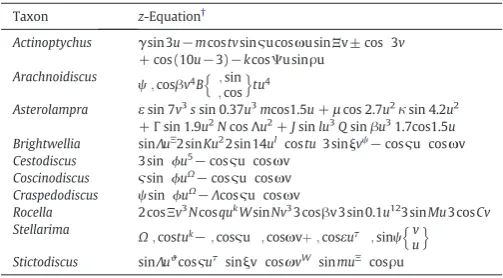
Published data fromHamm et al. (2003)are used for force values and their relationship to particular taxa and their maximum diameter or length. A plot of this relationship was devised, and a negative exponential function is used as a least squares best-fit curve ofy= 950.83e−0.018x_withR2_{= 0.9345 whereCoscinodiscus graniiGough is} used as the reference taxon at which the function must converge (Fig. 1). FromFig. 1, diatoms with heavier ornamented, rougher tex-tured surfaces require more force to break than smoother surfaces withfine features. That is, texture is 3D surface quality in terms of roughness, graininess, smoothness, or any other descriptor about the peaks, valleys and saddles that are geometrically characteristic of the surface of the diatom. The surface area of a largest possible patch on the diatom valve face is calculated via the results obtained for morpho-logical complexity. Stress on the surface area is calculated using Hooke's Law and is used as a measurement of functional complexity of the 3D surface. For more details on methods of calculation, see theAppendix A.

2.3. Multivariate complexity analysis

Matrices of morphological and functional complexity values, are ag-gregated using external unfolding analysis (Coombs, 1964; Heiser, 1987) based on multidimensional scaling (MDS) (Heiser, 1987) to cre-ate complexity gradients. The multivaricre-ate technique folds different types of data onto their ideal points so that the map that results depicts approximate distances among taxon complexities. Trade-offs among taxa and their complexity attributes are calculated as transformed prox-imities to produce a low dimensional complexity spatial map as com-plexity gradients of taxa over time. Eocene and Oligocene taxa can be combined as average proximities to assess morphological, functional and total complexity. The resultant gradients will rank the morpholog-ical, functional and total complexities as the change in complexity from the Eocene to Oligocene as a vector of taxa over time. For more details, see theAppendix A.

2.4. Magnitude and rate of complexity change

Using total complexity results as initial conditions, complexity change can be simulated to occur over a long period of time culminating in a steady-state system via afinite discrete Markov chain. At equilibri-um the expectation is that probability values will attain the same value across all taxa. If differences between initial andfinal states are detected, then changes of increasing or decreasing probability values are an indi-cation of increasing or decreasing complexity. The hypotheses to be Fig. 1.Load vs. diameter afterHamm et al.'s (2003)data.Coscinodiscus graniiis used as a reference point from with respect to the best-fit curve. Taxa plotted from left to right are:Fragilariopsis kerguelensis,Thalassiosira punctigera(50μm),T.punctigera(100μm), andCoscinodiscus graniiwherey=950.83e−0.018x

tested are:H0: Complexity does not change over time;HA1: Complexity increases over time;HA2: Complexity decreases over time.

Taxon complexity shifts occur as a_finite number of probable transi-tions. At each step, change in state (=taxon) is represented by the prob-ability that the new state (=another taxon) occurs only with reference to the just current state. The history of previous changes are not a factor in a Markov process, and the expected outcome is a mean number of steps to achieve each state where ultimately over a long period of time, equilibrium (stationary probability distribution) is reached. In the long run, magnitude of complexity change at equilibrium is mea-sured as a distance metric between initial andfinal states of the Markov chain. In the short run, meanfirst passage time as the magnitude of complexity change is the time it takes to get from the initial complexity state to each subsequent complexity state, culminating in arrival at the equilibrium complexity state. The length of time is a measure of the short term behavior between complexity states. The more transition states needed to get from one state to another, the higher the mean first passage time. The rate of complexity change can be determined by a plot of the taxon rank-ordered total complexity gradient versus total complexity transition states for each taxon. A least-squares best-fit curve is determined, and the slope of the curve is the rate of total complexity change. For more details, see theAppendix A.

2.5. Complexity change over time: driven or random trend?

To determine the mode of complexity change over time, structural equation modeling (SEM) (Pearl, 2000) is used. Originally used by Wright (1921), SEM involves a group of inferentially related variables in a graphical depiction of those relationships with respect to the causal assumptions used to devise the model. Causal analysis is used to model changing events and the actual and potential conditions under which such events might occur (Pearl, 2009). In causal inference, confounding bias as untested assumptions, unobserved factors, or non-experimental data can be taken into account (Pearl, 2000, 2009). SEM can include in-dependent variables becoming in-dependent variables as well as the re-verse (Pearl, 2000) and be both a cause and an effect in the same model (e.g.,Bowen and Guo, 2012; Pearl, 2000).

Causal inference can be used to determine whether a driven or random evolutionary trend is exhibited by centric diatom genera at the EOT. Each type of trend can be characterized via probability values. For a driven trend, centric diatom taxon complexity follows a time-directed trajectory so that those taxa occurring in the Oligocene have a complexity probability of 1, and those taxa occurring in the Eocene have a complexity probability of 0. To represent a random trend, Bernoulli sampling at the 0.1, 0.25, 0.4, 0.5, 0.6, 0.75, and 0.95 levels is used to randomly assign a probability of 0 or 1 to a given taxon. The pro-portion of 0 s to 1 s for the entire taxon data set is dictated by the level of Bernoulli sampling.

For input data, total complexity measurements are used in SEM. The Jacobian determinant is used as morphological complexity, and the Cauchy traction data extracted from Fig. 1are used as non-orthonormalized functional complexity measures for taxa. Each data set is square root transformed to approximate a multivariate normal distribution, and this rescaling insures that no category of data exerts undue influence in SEM. Time is represented as categorical variables so that Eocene is represented by 0 since it always precedes the Oligo-cene which is represented by 1. To test for a driven or random trend as potential outcomes, probabilities represent counterfactual condi-tionals (Pearl, 2000) of complexity change over time.

Counterfactuals enable the consideration of potential outcomes which can be characterized by“What if…”statements (Pearl, 2000) alongside actual outcomes (Neyman, 1923; Rubin, 1974).“Driven”or

“Random”are counterfactual to each other in SEM. Counterfactuals are conditional statements that can be focused into hypotheses to be tested with respect to evolutionary trends:H0: Complexity change over time is

a random evolutionary trend;HA: Complexity change over time is a driven evolutionary trend.

In SEM, the different types of variables are combined into a single analysis and depicted as a path diagram representing the structural part of the model. Such graphs can be models of predictions and inter-ventions (Pearl, 2000). Predictions involve cause and direct effect. Inter-ventions produce indirect effects, including insertion or deletion of observations, action or observation exchange, insertion or deletion of actions (Pearl, 2000), and act as confounding variables or paths (e.g.,Pearl, 2000, 2009). Connections representing predictions and in-terventions are represented by unidirectional arrows as causes, and bi-directed arrows representing associations (Pearl, 2000). Causal dia-grams structured such that the effects are identifiable will have a mini-mal number of path connections that are stable (Pearl, 2000). An acyclic directed graph is a causal diagram that has mutually independent error variances and is a well-structured model having the Markovian proper-ty (Pearl, 2000).

Causal connections can be made between endogenous and exoge-nous variables which may be observed or unobserved. Endogeexoge-nous var-iables are potential or realized effects and are influenced by other variables. Exogenous variables not influenced by other variables such as error variances that serve as background influences on the outcomes of endogenous variables (Pearl, 2000). Observed variables are directly measured and are also indicator variables. Unobserved variables and their relationship to observed variables constitutes the measurement part of SEM (e.g.,Bowen and Guo, 2012).

In graphical SEM, vertices are drawn as rectangles representing en-dogenous observed variables and ovals representing enen-dogenous unob-served variables. Exogenous unobunob-served variables represented by small circles are attached at the base of a unidirectional arrow. Means, vari-ances, regression weights, and intercepts can be assigned values as con-straints in SEM or left to vary freely, depending on the minimality and stability levels achieved in attempting tofit a structural model using max-imum likelihood or a least-squares approach (Bowen and Guo, 2012). Constraints are used to produce a causal path diagram that enables the es-timation of interventions and/or counterfactuals for predictions (Pearl, 2000). Interventions and counterfactuals can be represented either as quantities via variables or actions as arrows (Pearl, 2000).

The counterfactual conditional,“Random,”representing random outcome as an evolutionary trend is represented by the statement,

“Evolutionary trend would be random had complexity changes from the Eocene to the Oligocene occurred by chance._”The counterfactual

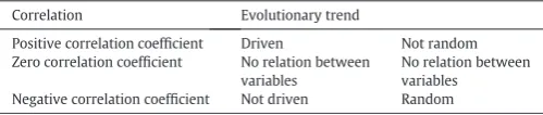
“Driven”representing driven outcome as an evolutionary trend is repre-sented by the statement,“Evolutionary trend would be driven had com-plexity changes from the Eocene to the Oligocene occurred in one direction.”In each model, the probability values for“Driven”indicate time-dependence where Eocene = 0 and Oligocene = 1 and for“ Ran-dom”indicate Bernoulli sampling, viz. 0 or 1 at levels from 0.1 to 0.95 that are assigned to each taxon. To decide if the null hypothesis should be rejected, correlation coefficients calculated for causally inferred rela-tionships among variables will be evaluated according toTable 1, where the largest correlation provides the decision on potential outcome. A positive correlation coefficient indicates a driven and non-random trend, a zero value indicates no relation between variables, and a nega-tive value indicates a non-driven and random trend. Non-random and non-driven trends may be fractal or chaotic and are not evaluated at

Table 1

Correlation coefficient categories for evaluation of results from structural equation model-ing (SEM).

Correlation Evolutionary trend

Positive correlation coefficient Driven Not random Zero correlation coefficient No relation between

variables

this time. Only a driven or random trend will be evaluated. For more de-tails on structural equation modeling, see theAppendix A.

3. Results

A total of 313 3D surface models were created for centric diatom genera from the Eocene and Oligocene. Each genus was represented by 31–33 models; examples are depicted inFig. 2. Jacobians were calcu-lated for each model from which each matrix was made square asym-metric using the cross product of the columns. Jacobian determinants were calculated and averaged for each genus as measurement of mor-phological complexity. Rank ordering the taxa indicates thatStictodiscus

is the most morphologically complex followed byActinoptychus,Rocella,

Asterolampra,Brightwellia,Coscinodiscus,Craspedodiscus,Cestodiscus,

Arachnoidiscus, and Stellarima, the least morphologically complex (Fig. 3). Thefive most morphologically complex taxa have more irregu-lar features on their valve faces than those with more reguirregu-lar valve face features. Morphological complexity change over time is mixed.

Functional complexity was calculated for each 3D diatom surface model as the Cauchy stress tensor using surface area of the valve face and interpolated scalar values of the Cauchy traction vector from Hamm et al.'s (2003)empirical load data (Fig. 4; least squares best-fit curvey= 950.62e−0.018x_withR2_{= 0.9982). The results were analyzed} using unidimensional external unfolding analysis (Fig. 5) where the so-lution was non-degenerate, having non-zero Kruskal's and Young's

STRESS values, a low De Sarbo's Index (1.2), and a Shepard's Index of 72% (Table 2andFig. 6) andfinal coordinates were averaged for each genus. Rank ordering indicated that highest functional complexity oc-curs with Asterolampra, followed by Arachnoidiscus, Rocella, and

Stictodiscus. These taxa exhibit multilayered structures on their valve face surfaces and have an irregularity to their surface features. Next in line going from more to less functional complexity areCestodiscus,

Coscinodiscus,Craspedodiscus andStellarima(Fig. 5). These genera have a more regular, repeating cross-hatching valve face surface, with finer cross-hatching occurring from more to less complex forms, respec-tively. The last two genera in line have very different valve face surfaces, withActinoptychushaving large smooth,flatter sections andBrightwellia

having a ring of holes surrounded byfinely textured regular features. For functional complexity, four of the Oligocene taxa occur near the head of the time arrow.

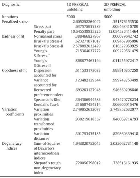
Total complexity was determined as the aggregation of morpholog-ical and functional complexity values using external unfolding analysis. The solution was non-degenerate, having non-zero Kruskal's and Young's STRESS values, a low De Sarbo's Index (2.0), and a Shepard's Index of 74% (Table 3andFig. 7), and unidimensionalfinal proximities were averaged for each diatom genus. Rank ordering of total complexity values follows a gradient similar to functional complexity with two ex-ceptions (Fig. 8).BrightwelliaandActinoptychustrade places so that total complexity is least forActinoptychus(Fig. 8). On a taxon-by-taxon basis, functional complexity contributes to total complexity change over time. Fig. 2.Diatom 3D surface models ofActinoptychus,Arachnoidiscus,Craspedodiscus,Cestodiscus,Stellarima(top row),Asterolampra,Brightwellia,Coscinodiscus,Rocella,Stictodiscus(bottom row).

Taxa were combined into an Eocene or Oligocene time bin for mor-phological, functional and total complexity using averaged proximities from external unfolding analysis. The percentages of the amount of con-tribution to each type complexity indicate that the Oligocene bin contains more complex taxa combined of which morphological complexity

contributes positively to this result (Fig. 9). Functional complexity indi-cates the opposite by contributing negatively to the Oligocene bin (Fig. 9).

3.1. Magnitude and rate of complexity change

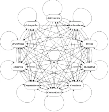
Using the results from external unfolding total complexity analysis, an initial probability transition probability matrix was calculated (Table 4) as input to produce afinite discrete Markov chain of ten cen-tric diatom genera from the Eocene or Oligocene (Fig. 10). The Markov chain is acyclic with no connection betweenActinoptychusat the start andAsterolampraat the end (Fig. 10). The Markov chain is irreducible, transient, non-absorbing, and reversible, and as all states are aperiodic and positive recurrent, the Markov chain is ergodic. As a result and using the Chapman–Kolmogorov equation relatingn-transition proba-bilities among all taxa, the stationary probability states are equivalent to the limiting probability states as the values of the Markov chain at equilibrium (Table 5).

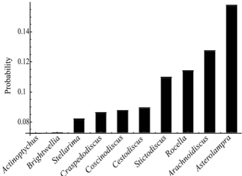
The stationary probability distribution indicates that transition from state to state as taxon shifts is exponential (Fig. 11). Equilibrium is achieved and verified by the normalized left eigenvector elements that sums to one for the eigenvalue equal to one. From the stationary distribution, initial complexity state atActinoptychusis 0.072. Subse-quently, the complexity transition values range from 0.073 for

Brightwelliato 0.08 forStellarima,Craspedodiscus, andCoscinodiscusto approximately 0.1 forCestodiscus,Stictodiscus, andRocellato 0.13 for Fig. 4.Combined force data with adjusted values for diatom 3D surface models. The least

squares best-fit curvey=950.62e−0.018x withR2

=0.9982 is based on the original curve (Fig. 1) usingCoscinodiscus graniias the reference point (130μm diameter) to convert patch surface areas to diameters based on the face of a cylinder with height = 1.

Fig. 5.Functional complexity based on Cauchy stress tensor values for each diatom genus from the averagefinal proximities from unidimensional external unfolding. Arrow points in the direction of least functionally complex,Brightwellia, to most functionally complex,Asterolampra, representing the Eocene or Oligocene.

Table 2

Diagnostics for 1D and 2D external unfolding analysis of functional complexity values.

Diagnostic 1D PREFSCAL

unfolding

2D PREFSCAL unfolding

Iterations 5000 5000

Penalized stress .659788856752 .522988312586

Stress part 2.276719864819 .019482682569

Penalty part 7.856230504374 14.038968922059

Badness offit Normalized stress .417915502470 .000379565312

Kruskal's Stress-I .646463844673 .019482435988

Kruskal's Stress-II 2.485296272389 .037385585377

Young's S-Stress-I .742137743428 .020417442640

Young's S-Stress-II .878613655667 .027157055296

Goodness offit Dispersion accounted for .582084497530 .999620434688

Variance accounted for .131812933801 .998859015639

Recovered preference orders .678548607942 .985993204524

Spearman's Rho .313899873360 .973227315183

Kendall's Tau-b .255336290642 .948715666859

Variation coefficients Variation proximities 2.468256953469 2.468256953469

Variation transformed proximities 1.008911927748 .736608150986

Variation distances .332685604713 .720682107040

Degeneracy indices Sum-of-squares of DeSarbo's intermixedness indices 1.523355677308 1.236062642009

Arachnoidiscusto 0.16 forAsterolampra. Overall, approximately twice as much time is spent inArachnoidiscusandAsterolamprastates as initial stateActinoptychus. At equilibrium, the more complex taxa,

ArachnoidiscusandAsterolamprapersist longer than the less complex taxonActinoptychus. When comparing Oligocene taxa to Eocene taxa, there is an increase in complexity of approximately 1.1 to 1.5 times the initial state ofActinoptychus(Fig. 11,Table 6).

The distance between initial transition andfinal stationary (limiting) probability matrices is calculated as a Frobenius norm of 0.019053. The

small positive change indicates an increase in total complexity that oc-curred in the long run for centric diatom genera across the EOT.

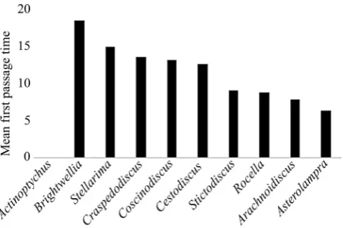
Meanfirst passage time decreases from least to most complex taxa (Fig. 12). More transitions are necessary, and therefore more time is used to get from the initial state,Actinoptychus, to two Eocene taxa—Brightwellia and Craspedodiscus—and three Oligocene taxa—Stellarima,Coscinodiscus, andCestodiscus—in contrast to the remaining taxa. The shortest transition period occurs from initial stateActinoptychusto more complex states,Stictodiscus,Rocella,

ArachnoidiscusandAsterolampra(Fig. 12). Transitioning from less to another less complex taxon is more time consuming than transitioning from less to more complex taxa. Taxon rank-ordered total complexity vs. total complexity transition states is depicted in Fig. 13. Least squares best-fit curve is ytrans= 1.4081x+ 85.087 (R2_{= 0.9543), with slope = 1.4081 as the rate of complexity change} over time.

From initial tofinal state at equilibrium, total complexity increases over time in the long run via discretefinite Markov chain analysis. More complex centric diatom genera are more likely to occur in the short run via meanfirst passage time, therefore complexity increases. From these analyses,H0andHA2are rejected.

3.2. Complexity change over time: driven or random trend?

A sample size of 313 3D surface models representing taxa from 10 centric diatom genera were used in SEM to determine mode of com-plexity trend. The theoretical causal structure of the model is character-ized by an evolutionary trend as an effect of complexity change which occurs as an effect over time. Unweighted least squares was used to cal-culate the discrepancy (χ2_{) function. Of the 100+ different models that} were created, 7 admissible models described the theoretical structure of the relationship of the variables had a stability index between 0 and 1. Minimality as minimum discrepancy (CMIN) yielded a best-fit model with lowest root mean square residual (RMR) and highest goodness-of-fit (GFI; AGFI; PGFI) statistics, reflecting a less penalized solution that is more parsimonious than others.

The best-fit structural model resulted in a path diagram of a recur-sive directed acyclic graph (Markovian) based on unweighted least squares representing the causal inference model (Fig. 14). Minimality and stability were achieved, and a permutation test of 500 iterations yieldedp= 0.002. Diagnostics indicated that Bernoulli sampling = 0.5 was the best-fit model (Table 6). All models tested were Fig. 6.2D external unfolding non-degenerate functional complexity space. SeeTable 2for diagnostic measures.

Table 3

Diagnostics for 1D and 2D external unfolding analysis of total complexity values.

Diagnostic 1D PREFSCAL

unfolding

2D PREFSCAL unfolding

Iterations 5000 5000

Penalized stress 2.605252264042 .351576153530

Stress part .637575933383 .009468416789

Penalty part 10.645538835326 13.054536411464 Badness offit Normalized stress .388466827967 .000089642742 Kruskal's Stress-I .623271071017 .009467985096 Kruskal's Stress-II 2.578092032429 .016322959925 Young's

S-Stress-I

.715364037772 .009229561479

Young's S-Stress-II

.868877463194 .011255972417

Goodness offit Dispersion accounted for

.611533172033 .999910357258

Variance accounted for

.123482129344 .999748753499

Recovered preference orders

.693283127948 .946569298646

Spearman's Rho .364306944583 .943470778234 Kendall's Tau-b .316687454314 .906600015476 Variation

coefficients

Variation proximities

2.749852632077 2.749852632077

Variation transformed proximities

.939219618337 .846069714793

Variation distances

.301793435185 .829860339418

Degeneracy indices

Sum-of-Squares of DeSarbo's intermixedness indices

1.943820752045 2.022062731149

Shepard's rough non-degeneracy index

unconstrained with regard to arrows between unobserved and ob-served endogenous variables.

The best-fit model (Table 6) resulted in 18 variables of 6 observed and 12 unobserved variables of which nine were endogenous and nine were exogenous (Fig. 14). There were 26 parameters where 17 hadfixed weights and nine error variances were set equal to one as input to constrain the model to be linear among unobserved endoge-nous variables. Forty-two sample moments were calculated with 6 un-constrained estimated parameters and 36 degrees of freedom.

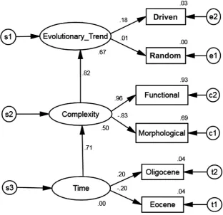
Regression weights as standardized estimates are labeled on each arrow in the path diagram (Fig. 15) and are an indicator of the stability of the model. Unobserved endogenous variables were highly correlated with direct effects from Time to Complexity (0.707) and from Complex-ity to Evolutionary Trend (0.816). Predictors explained the variance at 50% for Complexity and 66.7% for Evolutionary Trend (Fig. 15). Time was correlated with indirect effects on Evolutionary Trend (0.577). Var-iance was not predicted for Time (Fig. 15). UsingTable 1, an overall evo-lutionary trend can be causally inferred from these results.

Regression weights between observed and unobserved endogenous variables from the path diagram indicated direct effects where Com-plexity and Functional comCom-plexity were highly positively correlated (0.965), while Complexity was highly negatively correlated with Mor-phological complexity (−0.831). Time indirectly was highly correlated with Functional complexity (0.682) and highly negatively correlated

with Morphological complexity (−0.588). Predictors explained the var-iance at 69% for Morphological complexity and 93.1% for Functional complexity. UsingTable 1, these results indicate that morphological and functional complexity are causally opposing evolutionary trends.

Eocene had a low negative correlation (−0.198) and Oligocene had a low positive correlation (0.113) with Time (Fig. 15). Driven had a low positive correlation with a small direct effect on Evolutionary Trend (0.099), while Random had a correlation near zero (0.012) and a negli-gible direct effect. Predictors for Eocene, Oligocene, Driven, and Random were in the range of 0 to 4%. Indirect effects for Driven on Time and Complexity were negligible (0.057 and 0.081, respectively) and for Ran-dom were near zero (0.007 and 0.010, respectively). UsingTable 1, an overall evolutionary trend as directly driven cannot be causally inferred. Residual covariances among observed endogenous variables were [−1, 1] and are sufficiently small so that implied correlations of all var-iables are approximately equal to actual correlations expected of the input variables indicating the minimality of the model. Implied correla-tions showed that Evolutionary Trend was highly positively correlated with Functional complexity (0.788) and highly negatively correlated with Morphological complexity (−0.679). Morphological complexity was highly negatively correlated to Functional complexity (−0.802) reinforcing the earlier result regarding regression weights. Observed endogenous variables implied correlations with each other had negligi-ble values ranging from −0.14 to 0.12. Using Table 1, implied Fig. 7.2D external unfolding non-degenerate total complexity space. SeeTable 3for diagnostic measures.

correlations indicate morphological and functional complexity as caus-ally inferred opposing evolutionary trends, reinforcing earlier results.

Subtracting the residual covariance matrix from the implied covariance matrix results in the sample matrix. From this, the sample correlation matrix indicated that Morphological and Functional com-plexity were highly negatively correlated (−0.838), Oligocene and Driven were highly positively correlated (1.000), and Eocene was highly negatively correlated (−0.818) with Oligocene and Driven. Functional complexity was positively correlated (0.205) while Morphological com-plexity had a smaller positive correlation with Driven (0.085). Function-al complexity was negatively correlated with Eocene (−0.356) and positively correlated with Oligocene (0.202). Morphological complexity had a correlation near zero with Eocene (0.001) and small positive cor-relation with Oligocene (0.085). Corcor-relations of Morphological com-plexity, Functional comcom-plexity, Eocene, Oligocene, and Driven with Random were very small values (−0.068, 0.011, 0.073, −0.022, −0.022, respectively). UsingTable 1, sample correlations indicate mor-phological and functional complexity to be inferred as weakly driven evolutionary trends, and the null hypothesis can be rejected.

4. Discussion

Initially, 3D surfaces of centric diatom genera were measured deter-ministically to assess morphological, functional, and total complexity. As such, parts did not have to be defined, and there was no need to refer to particular descriptors, negation terms or qualifiers. Rather than relying on quantity via counting, quality of 3D surface morpholog-ical features was used to measure complexity and provide a natural link between form and function. It was shown that complexity is measurable as a multivariate quantity. Each type of complexity is multivariable, en-abling multiple measurements to be consolidated into specific complex-ity values in determiningn-dimensional complexity.

Measurement of the magnitude and mode of complexity as an evo-lutionary trend was accomplished within probability (Markovian) frameworks. Finding complexity to be a dynamical, ergodic system could be used as predictive values to enable projection of trends beyond the results given. Given the results of this study, for example, increasing total complexity and functional complexity (unlike morphological com-plexity) as a driven trend may be projected to be true throughout the Cenozoic to the recent. Probabilistic frameworks presented here could be used with additional taxa to test whether the trends are maintained, and if not, what hypotheses may emerge as relevant for testing.

Additional diatom taxa could be used in an extension of the current study. From diatom biostratigraphy of the Late Oligocene to the Quaternary,CestodiscusandCoscinodiscusare prevalent along with mor-phologically similar Actinocyclus Ehrenberg (Barron, 1985), and

AsteromphalusEhrenberg is present (Barron, 1985) which is morpho-logically similar toAsterolampra. The very large genus ofThalassiosira

P. T. Cleve is well represented, especially in the Pliocene onward Fig. 9.Comparison of combined taxa Eocene and Oligocene bins for morphological, func-tional and total complexity.

(Barron, 1985), and somewhat similar in valve face geometric texture to

Stellarima.

Throughout the Cenozoic into the Quaternary, other stratigraphically important taxa (e.g.,Barron et al., 2015), both centric and pennate, in-clude Hemiaulus Ehrenberg, Clavularia Greville, Cavitatus jouseana

(Sheshukova-Poretskaya) Williams,TriceratiumEhrenberg,Rhizosolenia

T. Brightwell,NitzschiaHassall,RouxiaJ. Brun and Héribaud-Joseph in Héribaud (Fenner, 1985; Barron, 1982/1983; Barron, 1985). The expecta-tion is that funcexpecta-tional complexity of the pennate taxa would be similar to

Fragilariopsis kerguelensiswith their position nearby on the load curve (Fig. 1). ForTriceratium, the expectation of functional complexity is a po-sition aboveThalassiosiraand below the pennates on the load curve (Fig. 1). From the result of this study, inferences about any diatom taxon position could be made, and whether any of these taxa would bol-ster or detract from the results of the current study would need to be tested.

Taxa such asHemiaulus(Eocene) andRhizosolenia(Miocene) have protrusions which may be construed to be morphologically complex at-tributes of frustule structure. As single cells,Rhizosoleniais lightly silici-fied compared to the more robustly silicifiedHemiaulus(Round et al., 1990) which may be viewed as more functionally complex. Protrusions are primarily used to form chains, and with both taxa, these protrusions are easily broken (Round et al., 1990). Predation resistance is unlikely to be functionally significant for these taxa, and therefore functional com-plexity would require a different measure with respect to ability to form colonies.

Complexity change was determined by looking at gradients of taxa per time as well as time bins of combined taxa. On a taxon-by-taxon basis, functional complexity was more important in total complexity (Figs. 5 and 8). By contrast, when looking at combined taxa in time bins, morphological complexity contributed more to total complexity (Fig. 9). Functional and morphological complexity occur in opposing ways, and these results were supported by causal inference analysis (Fig. 15). That morphological and functional complexity may exhibit op-posing trends has been determined in previous studies (e.g.,McShea and Hordijk, 2013).

Functional complexity was found to be a driver of increase in plexity change as an evolutionary trend. An increase in functional com-plexity may induce a decrease in environments selecting for increasing morphological complexity (Auerbach and Bongard, 2014). Morphologi-cal complexity may not increase in complex environments if the cost is too high (Auerbach and Bongard, 2014), and higher morphological complexity is not necessarily equivalent to evolutionary complexity and success (McNamara, 2006).

in functional separation and the potential for novelties in organismal form (Alfaro et al., 2004; Wainwright, 2007). Highly different morphol-ogies can produce the same functionality (Alfaro et al., 2004; Wainwright, 2007) which facilitates phenotypic diversification (Wainwright, 2007). Centric diatoms from the Eocene and Oligocene may be exhibiting this pattern.

Diatom morphological changes have been closely linked to environ-mental changes (Round et al., 1990), and distributional patterns were affected by environmental changes during the EOT (Jordan and Stickley, 2010; Gladenkov, 2014). In the Early Cretaceous, diatoms were more environmentally tolerant, had more complicated and variable life cycles (Harwood et al., 2007), and by the Early Eocene were cosmopolitanly distributed (Fenner, 1985; Harwood et al., 2007). Oceanic circulation was influenced by equatorial patterns with relatively warm bottom wa-ters and broad upwelling events with locally high biogenic silica depo-sition in upwelling regions (Barron and Baldauf, 1989; Baldauf and Barron, 1990). In the Middle Eocene, species with robust, heavily silici-fied frustules were present, and widespread biogenic silica deposition occurred because of an intensive increase in oceanic circulation via in-creased tectonic activity (Baldauf and Barron, 1990). As a result, surface water productivity increased with increasing coastal and equatorial up-welling activity (Barron and Baldauf, 1989; Baldauf and Barron, 1990), and diatom assemblages generally became more provincial (Fenner, 1985). By the late Middle Eocene, polar cooling accelerated, latitudinal thermal gradients became more pronounced, and increased stratifi ca-tion occurred (Barron and Baldauf, 1989; Baldauf and Barron, 1990; Zachos et al., 2008).

Continued cooling occurred in the earliest Oligocene, and biogenic silica deposits increased in the Southern Oceans and decreased in the middle latitudes (Barron and Baldauf, 1989; Baldauf and Barron, 1990). In the low latitudes, upwelling events became well established, oceanic circulation continued to intensify, and diatoms continued to be provincial (Fenner, 1985). In the Late Oligocene, biogenic silica depo-sition increased in some areas, but sediments in the equatorial Paci_fic were devoid of diatom frustules (Barron and Baldauf, 1989). An increase in taxa withfinely silicified frustules emerged as heavily silicified forms decreased (Fenner, 1985; Barron and Baldauf, 1989) as biogenic silica deposition changed in magnitude from the Atlantic to Pacific and South-ern Oceans (Barron and Baldauf, 1989).

Turbulence in the oceanic water column for brief periods spurred di-atom productivity to ensure that didi-atoms dominated the Cenozoic (Katz et al., 2004). Rapid evolutionary response (Jordan and Stickley, 2010) via selectivity led to the rise and success of diatoms (Katz et al., 2004). Episodic nutrient availability was capitalized on by diatoms because of their ability to acquire and store resources (Katz et al., 2004). During

Ta b le 5 Lim iting pro b ab ility ma trix of to ta l comp lex ity fi n ite d isc re te M ar k ov ch ai n o f 1 0 cen tr ic d iat om ta xa . Actinoptychus Brightwellia Stellarima Craspedodiscus Coscinodiscus Cestodiscus Stictodiscus Rocella Arachnoidiscus Asterolampra Actinoptychus 0.147614 0.147613 0.147614 0.147613 0.147614 0.147613 0 0 0 0 Brightwellia 0.147001 0.147001 0.147001 0.147001 0.147001 0.147001 0.001286 0.001286 0.001286 0.001286 Stellarima 0.13108 0.13108 0.13108 0.13108 0.13108 0.13108 0.034725 0.034725 0.034725 0.034725 Craspedodiscus 0.123724 0.123724 0.123724 0.123725 0.123724 0.123724 0.050173 0.050173 0.050173 0.050173 Coscinodiscus 0.121387 0.121386 0.121386 0.121387 0.121386 0.121386 0.055083 0.055083 0.055083 0.055083 Cestodiscus 0.118108 0.118108 0.118108 0.118108 0.118108 0.118108 0.061968 0.061968 0.061968 0.061968 Stictodiscus 0.083077 0.083077 0.083077 0.083077 0.083077 0.083077 0.135543 0.135543 0.135542 0.135543 Rocella 0.075624 0.075624 0.075624 0.075624 0.075624 0.075624 0.151195 0.151195 0.151195 0.151196 Arachnoidiscus 0.052386 0.052386 0.052386 0.052386 0.052386 0.052386 0.200002 0.200001 0.200002 0.200001 Asterolampra 0 0 0 0 0 0 0.310025 0.310026 0.310026 0.310025

the Eocene and Oligocene, major diatom turnover events occurred to change the composition of assemblages in response to changing cli-mates (Barron and Baldauf, 1989; Baldauf and Barron, 1990), sea levels, ice advancement, and atmospheric CO2levels (Jordan and Stickley, 2010). Diatoms prospered in shallow waters on continental margins and have changed the structure of marine food webs (Katz et al., 2004). From the current study, the composition of diatom taxa that oc-curred throughout the Eocene and Oligocene changed in complexity.

Actinoptychus, a morphologically complex genus (Fig. 3), occurred in the Late Cretaceous into the Eocene (Baldauf and Barron, 1987; Harwood and Nikolaev, 1995). Along with the less morphologically complexCraspedodiscus(Fig. 3) in the Early to Middle Eocene, morpho-logically complexAsterolampraandBrightwellia(Fig. 3) were prevalent (Fenner, 1985).Arachnoidiscus, a morphologically less complex genus having a regular surface pattern (Fig. 3), was abundant as well during this time (Fenner and Mikkelsen, 1990). By the end of the Middle Eo-cene, the less common species ofCraspedodiscusdisappeared, and by the Middle to Late Eocene, althoughAsterolampra,Brightwellia, and

Craspedodiscusstill dominated, many common and typical Eocene taxa disappeared in the Middle Oligocene (Fenner, 1985). In the Early Oligo-cene, cosmopolitan species were still present, and at the Eocene– Oligo-cene boundary, the less complex genus,Cestodiscus(Fig. 3) had species that became endemics. Cosmopolitan species of the morphologically less complex genus,Coscinodiscus, and the more complex genusRocella

(Fig. 3)first appear and became common during the Middle Oligocene (Fenner, 1985).

With increasing cooling and oceanic turbulence along with increased tectonic activity producing increases in productivity and di-versi_fication from the Eocene to the Oligocene, environmental and cli-mate change resulted in more complex ecological habitats for diatoms (Katz et al., 2004; Jordan and Stickley, 2010). Environmental specificity and adaptability of diatoms (Harwood et al., 2007) may indicate ecospace differentiation and expansion to accommodate the change

from cosmopolitan to more provincial and endemic taxa. Taking advan-tage of the expansion of ecospace induces an increase in ecological com-plexity (Knoll and Bambach, 2000) which may be a response to changing latitudinal, bathymetric, hydrodynamic, and temperature gra-dients. The cost of even slightly increasing complexity may be accept-ably borne in terms of ability to acquire nutrients and resources in changing environmental and climate conditions. Such costs may induce the adaptation of specific diatom taxa to specialized environments.

Selectivity of predation resistance is evident in centric diatom mor-phologies (Smetacek, 2001). Selecting for predation resistance should cause more complex morphologies to evolve than what might happen by chance (Auerbach and Bongard, 2014). However, mechanical com-plexity decreases in environments that select for increasing morpholog-ical complexity (Auerbach and Bongard, 2014) so that morphologmorpholog-ical complexity may decrease as a response to increasing functional com-plexity (McShea and Hordijk, 2013). This may be inferred with centric diatom genera from the Eocene and Oligocene by the current study. By the time of the turnover event at the EOT,Brightwelliabecame extinct as did many species ofActinoptychus,Arachnoidiscus,Asterolampra, and

Craspedodiscus, so that these Eocene taxa were unavailable as food for predators. Oligocene taxaRocella,Stictodiscusand many species of

Cestodiscus, andStellarimabecame extinct as another turnover event from the Middle to Late Miocene occurred with the proliferation of pen-nate diatom taxa (Strelnikova, 1990). The net result is a loss of morpho-logically complex centric taxa over time, yet more predation resistance is necessary because increasing ecological complexity provided an

Fig. 12.Meanfirst passage time from the initial state,Actinoptychus, to each succeeding state (=taxon) in the process of changing complexity. Each successive state has fewer transitions than the preceding state.

Fig. 13.Plot of taxon rank-ordered total complexity vs. total complexity transition states from meanfirst passage times from discretefinite Markov chain. Least squares best-fit curve isytrans=1.4081x+85.087 withR2=0.9543; the slope = 1.4081 and is the rate of complexity change over time.

Table 6

Best-fit diagnostics for SEM models. All models are unconstrained with Bernoulli sampling used to assign probability 0 or 1 to each taxon. Best-fit parameters measured are as follows: NPAR is the number of estimated parameters, CMIN is the minimum discrepancy, RMR is root mean residual, GFI is goodness-of-fit, AGFI is adjusted goodness-of-fit, and PGFI is parsimo-nious goodness-of-fit. Best-fit model used for analysis is Bernoulli sampling = 0.5.

Model NPAR CMIN RMR GFI AGFI PGFI

Bernoulli sampling = 0.1 6 508.457 .375 .988 .987 .847

Bernoulli sampling = 0.25 6 489.740 .367 .989 .987 .848

Bernoulli sampling = 0.4 6 471.892 .359 .989 .988 .848

Bernoulli sampling = 0.5 6 468.681 .358 .989 .988 .848

Bernoulli sampling = 0.6 6 470.861 .359 .989 .988 .848

Bernoulli sampling = 0.75 6 483.943 .364 .989 .987 .848

Fig. 14.SEM of labeled causal inference diagram for centric diatom genera and evolutionary trend of complexity. Path from unobserved endogenous variables Time to Complexity to Evo-lutionary Trend is constrained to be linear (regression weights = 1). All exogenous variables are set to error variances = 1 and constrained to be linearly related to unobserved endogenous variables. Observed endogenous variables are unconstrained. Driven and Random are probability vectors that are counterfactual to each other.

avenue for increasing abundances of Cenozoic marine invertebrates, which in turn induced large changes in marine food webs (Katz et al., 2004).

Limiting nutrient conditions in the oceans have changed the de-gree of silicification of diatom frustules but has not prevented diatom diversification (Harwood et al., 2007; Jordan and Stickley, 2010). In general, diatom genera richness is highly correlated with Cenozoic invertebrate richness (Katz et al., 2004). Increased quality and quantity of primary producers during the Cenozoic has influenced marine invertebrate evolution (Katz et al., 2004). Coevolution of di-atom taxa and some predators may be evidence of a driven response (Smetacek, 2001; Michels et al., 2012). For some copepods, silica coating on their chitinous teeth is a coevolved trait with diatoms (Katz et al., 2004; Michels et al., 2012). Few studies exist on preda-tion resistance at the scale of diatoms, and invertebrate grazers are inferred to be species specific in terms of head size relative to diatom size (Tall et al., 2006a, 2006b).

For centric diatoms across the EOT, all have differing morphologies yet all have some degree of predation resistance (Hamm, 2005). Plank-ton evolution is generally driven by predator–prey interactions rather than competition (Smetacek, 2001). The variety of morphologies of the diatom frustule is a reflection of predation resistance as a unifying functionality rather than competitive advantage among diatom taxa (Smetacek, 2001). However, as diatoms inhabit more specific habitats (e.g.,Round et al., 1990; Lowe, 2011) over the long term, this situation may place limitations on the kinds of diatoms that are available to pred-ators in a given area. Nutritional value of protein, lipids and carbohy-drates vary in different diatom taxa (Lowe, 2011). Predators may occupy specific habitats which may restrict their access to highly nutri-tious diatoms (Lowe, 2011). Some diatoms may avoid predators by ver-tically descending in the water column at night to acquire nutrients, then vertically ascending during daylight to photosynthesize (Katz et al., 2004). All of these factors could put selective pressure on predators.

Rapid evolution of diatoms during the Eocene and Oligocene oc-curred in response to environmental and climate conditions, increas-ing diatom environmental specificity and the proliferation of endemic and provincial taxa. Selecting for predation resistance might occur as a constraint on the kinds of predators adapted to the specific habitats now occupied by diatoms during this time. Functional efficiency (McShea and Hordijk, 2013) may be more a re-sult of changing ecological complexity rather than morphological complexity. Ecological complexity over the long term increases as a directional pattern, and functional complexity should do so as well

(Knoll and Bambach, 2000). Morphological complexity changes in response to ecological complexity, yet need not be increasing or driven. Morphological and functional complexity change may re-spond in opposing, unconnected ways to ecological complexity.

5. Conclusions

Using 3D surface models of centric diatom genera, morphological and functional complexity was analyzed as multivariate quantities. Markov chain analysis enabled a probabilistic framework in which to measure multivariate total complexity as increasing across the EOT. Functional complexity on a taxon-by-taxon basis contributed to in-creasing total complexity. Combined taxa in Eocene or Oligocene bins indicated that morphological complexity contributed to increasing total complexity. Functional complexity does not need to increase with increasingly complex morphologies or vice versa. From causal in-ference analysis, morphological and functional complexity exhibited weakly driven evolutionary trends. Changes in environmental and cli-mate conditions across the EOT may have induced predation resistance as an ecological response differently when looking at morphological in contrast to functional complexity as macroevolutionary patterns over time.

Acknowledgements

I would like to thank Daniel J. Miller for his thoughtful and insightful comments that improved this manuscript. I would also like to thank two anonymous reviewers and Richard Jordan for their very helpful com-ments that also improved this manuscript. No external funding sources or resources contributed to this study.

Appendix A

A.1. Methods

A.1.1. Selection procedure of taxa for inclusion in complexity analysis

I define all possible surface morphological patterns to be the pool from which to select samples,s. Prior knowledge,Z, consists of types ofn-surface morphological patterns for Coscinodiscales, Stictodiscales, Arachnoidiscales, and Asterolamprales given asZ1,Z2,Z3,Z4, respective-ly. The values to be determined are the genera,Y, that have thei, 1, 2,…,

n-surface morphological patterns.

The selection indicator variable for samples s1, s2, s3, s4 is As = (A1, A2, …, An)T. The sampling scheme to select genera

from As is

n _A

i¼1;i∈s

otherwise;Ai¼0;i∈s. Sampling is accomplished

ac-cording to the rule used to evaluate A and is given as

f(AS| Z,Y;Φ) where Φis an unknown parameter (Smith, 1983).

FromZ, the rule for genus selection is: the valve face shape approxi-mates circularity and has radiating areolae reflecting radial symmetry. The sampling scheme is based only onZso that any genus,Yi, can be selected viaAs. That is in probability terms,P(Y=y,A=a|Z= z) =P(Y=y|Z=z) P (A=a|Z=z). In effect, the rule becomes

f(As|Z;Φ), and the sampling selection process satisfies conditional

independence and the ignorability criterion (Dawid, 1979; Smith, 1983; Pearl, 2000, 2009).

A.2. Morphological complexity

Partial derivatives numerically solved from parametric 3D equations with boundary conditions [0, 2π] become elements of the Jacobian ma-trix (Jacobian) (Pappas, 2005a, 2005b, 2008; Pappas and Miller, 2013). Parametric 3D equations are a vector mapping F(u,v) =

f[x(u,v),y(u,v),z(u,v)] withF(x,y,z) =F[f(u,v),g(u,v),h(u,v)]so that tangent planesF(u,v) =F(x,y,z)for one dimension. Similarly, tangent planes for the other two dimensions as G(u,v) =G(x,y,z) and Table 7

‡_{Terms with parameters and coefficients of thez-equation for each centric diatom genus.} For all parameters,u,v∈[0,2π].

Taxon z-Equation†

Actinoptychus γsin 3u−mcostvsinςu cosωu sinΞv± cos 3v + cos (10u−3)−kcosΨu sinρu

Arachnoidiscus

ψ;cosβv4_Bn;sin

;cos o

tu4

Asterolampra εsin 7v3

ssin 0.37u3

mcos1.5u+μcos 2.7u2_κ sin 4.2u2 +Γsin 1.9u2

NcosΛu2 +Jsinlu3

Qsinβu3 1.7cos1.5u Brightwellia sinΛu2 sinKu2

2 sin14ul

costu3 sinξvψ−cosςu cosωv Cestodiscus 3 sin ϕu5_{−cosςu cosωv}

Coscinodiscus ςsin ϕuΩ_{−cosςu cosωv}

Craspedodiscus ψsin ϕuΩ−Λcosςu cosωv Rocella 2 cosv3

Ncosquk

WsinNv3

3 cosβv 3 sin 0.1u12

3 sinMu3 cosCv Stellarima _Ω;

costuk_{−;cosςu ;cosωvþ;cosεu}τ _;sinψnv

u o

Stictodiscus sinΛuϑcosςuτsinξv cosωvW _sinmucosρu

‡ _{See text forx- andy-equations.}

† _{Coefficients: 0≤ε≤2, 0≤β≤4.3, 0.1≤μ≤0.4, 0.1≤κ≤1, 0.1≤q≤2, 0.2≤m≤1.6, 0.2≤}

Λ≤4, 0.4≤Γ≤0.7, 0.5≤γ≤2, 0.6≤ϕ≤1, 0.7≤J≤2.5, 0.7≤L≤8, 1≤τ≤2, 1≤W≤3, 1≤ψ≤