R E S E A R C H
Open Access
A modified regularization method for
finding zeros of monotone operators in
Hilbert spaces
Prasit Cholamjiak
1, Watcharaporn Cholamjiak
1and Suthep Suantai
2**Correspondence:
[email protected] 2Department of Mathematics,
Faculty of Science, Chiang Mai University, Chiang Mai, 50200, Thailand
Full list of author information is available at the end of the article
Abstract
We study the regularization method for solving the variational inclusion problem of the sum of two monotone operators in Hilbert spaces. The strong convergence theorem is then established under some relaxed conditions which mainly improves and recovers that of Qinet al.(Fixed Point Theory Appl. 2014:75, 2014). We also apply our main result to the convex minimization problem, the fixed point problem and the variational inequality problem. Finally we provide numerical examples for supporting the main result.
MSC: 47H09; 47H10
Keywords: convex minimization problem; maximal monotone operator; inverse strongly monotone operator; regularization method; variational inequality problem
1 Introduction
LetCbe a nonempty subset of a real Hilbert spaceH. Define the domain and the range of an operatorB:H→HbyD(B) ={x∈H:Bx= ∅}andR(B) ={Bx:x∈D(B)}, respec-tively. The inverse ofB, denoted byB–, is defined byx∈B–yif and only ify∈Bx. We
study the problem of findingxˆsuch that
∈Axˆ+Bxˆ,
whereA:C→H is an operator andB:D(B)⊂H→H is a set-valued operator. This problem is called the variational inclusion problem. Some typical problems arising in var-ious branches of science, applied sciences, economics, and engineering such as machine learning, image restoration, and signal recovery can be viewed as this form. To be more precise, it includes, as special cases, the variational inequality problem, the split feasibility problem, the linear inverse problem, and the following convex minimization problem:
min
x∈HF(x) +G(x),
whereF:H→Ris a smooth convex function, andG:H→Ris a non-smooth convex function. That is,
F(xˆ) +G(xˆ) =min
x∈HF(x) +G(x) ⇔ ∈ ∇F(xˆ) +∂G(xˆ),
where∇Fis the gradient ofFand∂Gis the subdifferential ofGdefined by
∂G(x) =z∈H: y–x,z+G(x)≤G(y),∀y∈H.
Forr> , define the mappingTr:C→D(B) as follows:
Tr= (I+rB)–(I–rA). (.)
We see that
Trx=x ⇔ x= (I+rB)–(x–rAx) ⇔ x–rAx∈x+rBx ⇔ ∈Ax+Bx,
which shows that the fixed points set ofTrcoincides with the solutions set of (A+B)–(). This suggests the following iteration process:x∈Cand
xn+= (I+rnB)–(xn–rnAxn) =Trnxn, n≥,
where{rn} ⊂(,∞) andD(B)⊂C. This method is called a forward-backward splitting algorithm [, ]. IfA≡, then we obtain the proximal point algorithm [–] and ifB≡, then we obtain the gradient method []. However, it is noted that the sequences generated by these schemes converge weakly in general. In the literature, many methods have been suggested to solve the variational inclusion problem for maximal monotone operators; see,e.g., [–].
Very recently, Qinet al.[] proved the following theorem in Hilbert spaces.
Theorem Q Let A:C→H be anα-inverse strongly monotone mapping and let B be a
maximal monotone operator on H.Assume that D(B)⊂C and(A+B)–()is nonempty. Let f :C→C be a fixed k-contraction and let Jrn= (I+rnB)–.Let{zn}be a sequence in C
in the following process:z∈C and
wn=αnf(zn) + ( –αn)zn,
zn+=Jrn(wn–rnAwn+en), n≥,
(.)
where{αn} ⊂(, ),{en} ⊂H,and{rn} ⊂(, α).If the control sequences satisfy the follow-ing restrictions:
(a) αn→, ∞
n=αn=∞and ∞
n=|αn+–αn|<∞;
(b) <a≤rn≤b< αand ∞
n=|rn+–rn|<∞;
(c) ∞n=en<∞.
Then{zn}converges strongly to a point x∈(A+B)–(),where x=P
(A+B)–()f(x).
In this paper, motivated by Qinet al.[], we prove that the above theorem still holds even if the additional conditions that∞n=|αn+–αn|<∞and
∞
n=|rn+–rn|<∞are
2 Preliminaries and lemmas
We now provide some basic concepts, definitions and lemmas which will be used in the sequel.
LetCbe a nonempty, closed, and convex subset of a real Hilbert spaceHwith norm · and inner product ·,·. For eachx∈H, there exists a unique nearest point inC, denoted byPCx, such thatx–PCx=miny∈Cx–y. ThenPCis called the metric projection ofH on toC. Forx∈H, we know that
x–PCx,y–PCx ≤ (.)
for ally∈C. Recall that the mappingT:C→Cis said to be (i) nonexpansive ifTx–Ty ≤ x–yfor allx,y∈C; (ii) k-contractive if there exists <k< such that
Tx–Ty ≤kx–y
for allx,y∈C; (iii) firmly nonexpansive if
Tx–Ty≤ x–y–(I–T)x– (I–T)y for allx,y∈C.
(iv) monotone if Tx–Ty,x–y ≥for allx,y∈C;
(v) α-inverse strongly monotone if there existsα> such that
Tx–Ty,x–y ≥αTx–Ty
for allx,y∈C. We denote byF(T)the fixed points set ofT, that is, F(T) ={x∈C:x=Tx}.
A set-valued operatorBis said to bemonotoneif, for eachx,y∈D(B),
u–v,x–y ≥, u∈Bx,v∈By.
A monotone operatorAis said to bemaximalifR(I+rB) =H for allr> (see Minty []). For a maximal monotone operatorBonH, andr> , we define the single-valued resolventJr:H→D(B) byJr= (I+rB)–. It is well known thatJris firmly nonexpansive, andF(Jr) =B–().
We now collect some crucial lemmas.
Lemma .[] Let C be a nonempty,closed,and convex subset of a real Hilbert space H. Let the mapping A:C→H beα-inverse strongly monotone and r> be a constant.Then we have
(I–rA)x– (I–rA)y≤ x–y+r(r– α)Ax–Ay
for all x,y∈C.In particular,if <r≤α,then I–rA is nonexpansive.
Lemma .[] Let C be a nonempty,closed,and convex subset of a Hilbert space H,and T:C→C be a nonexpansive mapping with F(T)=∅.If xnx andxn–Txn →,then x∈F(T).
Lemma .[] Let{an}and{cn}are sequences of nonnegative real numbers such that
an+≤( –δn)an+bn+cn, n≥,
where{δn}is a sequence in(, )and{bn}is a real sequence.Assume∞n=cn<∞.Then the following results hold:
(i) Ifbn≤δnMfor someM≥,then{an}is a bounded sequence. (ii) If∞n=δn=∞andlim supn→∞bn/δn≤,thenlimn→∞an= . We need the following crucial lemma proved by He-Yang [].
Lemma .[] Assume{sn}is a sequence of nonnegative real numbers such that
sn+≤( –γn)sn+γnδn, n≥ and
sn+≤sn–ηn+ρn, n≥,
where{γn}is a sequence in(, ),{ηn}is a sequence of nonnegative real numbers and{δn},
and{ρn}are real sequences such that (i) ∞n=γn=∞,
(ii) limn→∞ρn= ,
(iii) limk→∞ηnk= implieslim supn→∞δnk≤for any subsequence{nk}of{n}.
Thenlimn→∞sn= .
3 Main results
In this section, we present the main theorem of this paper.
Theorem . Let A:C→H be anα-inverse strongly monotone mapping and let B be a maximal monotone operator on H such that D(B)⊂C and(A+B)–()is nonempty.Let
f :C→C be a k-contraction.Assume that{αn} ⊂(, ),{en} ⊂H,and{rn} ⊂(, α)with the following restrictions:
(a) αn→and ∞
n=αn=∞; (b) <a≤rn≤b< α;
(c) ∞n=en<∞oren/αn→.
Then the sequence{zn}generated by(.)converges strongly to a point x∈(A+B)–(), where x=P(A+B)–()f(x).
Proof Let{xn}be a sequence generated byx∈Cand
yn=αnf(xn) + ( –αn)xn,
Firstly, we shall show that{xn}and{zn}are equivalent. Indeed,
yn–wn=αn
f(xn) –f(zn)+ ( –αn)(xn–zn)
≤αnkxn–zn+ ( –αn)xn–zn
= –αn( –k)xn–zn.
Using Lemma ., condition (b), and the fact thatJrnis nonexpansive, we obtain
xn+–zn+=Jrn(yn–rnAyn) –Jrn(wn–rnAwn+en) ≤(yn–rnAyn) – (wn–rnAwn+en) ≤ yn–wn+en
≤ –αn( –k)xn–zn+en.
Applying Lemma .(ii) with conditions (a) and (c), we conclude thatxn–zn →. On the other hand, it can be checked thatP(A+B)–()f is a contraction. So there exists a
unique pointx∈Csuch that
x=P(A+B)–()f(x). (.)
To finish our proof, it suffices to show thatxn→xasn→ ∞.
We next show that{xn}is bounded. Fixingp∈(A+B)–(), we obtain
yn–p=αn
f(xn) –f(p)
+αn
f(p) –p+ ( –αn)(xn–p)
≤αnkxn–p+αnf(p) –p+ ( –αn)xn–p
= –αn( –k)
xn–p+αnf(p) –p.
It follows that
xn+–p=Jrn(yn–rnAyn) –Jrn(p–rnAp)
≤ yn–p ≤ –αn( –k)
xn–p+αnf(p) –p.
Hence{xn}is bounded by Lemma .(i). So are{f(xn)}and{yn}. Observing
yn–x =αnf(xn) –f(x),yn–x
+αnf(x) –x,yn–x
+ ( –αn) xn–x,yn–x
≤αnkxn–xyn–x+αnf(x) –x,yn–x
+ ( –αn)xn–xyn–x
= –αn( –k)xn–xyn–x+αnf(x) –x,yn–x
≤
–αn( –k)xn–x+yn–x
+αnf(x) –x,yn–x
,
we have
yn–x≤
– αn( –k) +αn( –k)
xn–x+
αn
+αn( –k)f(x) –x,yn–x
So, by Lemma . and the firm nonexpansiveness ofJrn, we have
xn+–x =Jrn(yn–rnAyn) –Jrn(x–rnAx)
≤(yn–rnAyn) – (x–rnAx)
–(I–Jrn)(yn–rnAyn) – (I–Jrn)(x–rnAx)
≤ yn–x–rn(α–rn)Ayn–Ax
–(I–Jrn)(yn–rnAyn) – (I–Jrn)(x–rnAx)
≤
– αn( –k) +αn( –k)
xn–x+
αn
+αn( –k)f(x) –x,yn–x
–rn(α–rn)Ayn–Ax
–(I–Jrn)(yn–rnAyn) – (I–Jrn)(x–rnAx)
.
This implies that
xn+–x≤
– αn( –k) +αn( –k)
xn–x+
αn
+αn( –k)f(x) –x,yn–x
(.)
and
xn+–x≤ xn–x–rn(α–rn)Ayn–Ax
–(I–Jrn)(yn–rnAyn) – (I–Jrn)(x–rnAx)
+ αn
+αn( –k)f(x) –xyn–x. (.)
We set, for all n≥ , sn =xn–x, γn = +ααnn(–(–kk)), δn =
–k f(x) –x,yn –x, ρn =
αn
+αn(–k)f(x) –xyn–x, and ηn =rn(α –rn)Ayn–Ax
+(I–J
rn)(yn–rnAyn) –
(I–Jrn)(x–rnAx). We can check that all sequences satisfies conditions (i) and (ii) in
Lemma .. Then (.) and (.) can be rewritten as the following inequalities:
sn+≤( –γn)sn+γnδn, n≥
and
sn+≤sn–ηn+ρn, n≥.
To complete the proof, we verify that the condition (iii) in Lemma . is satisfied. Let {nk} ⊂ {n}be such thatηnk→. Then, by condition (b), we have
lim
n→∞Aynk–Ax=
and
lim
Hence we obtain
lim
n→∞ynk–Jrnk(ynk–rnkAynk)= .
By Lemma .(ii) and (b), we have
Ja(ynk–aAynk) –ynk≤Jrnk(ynk–rnkAynk) –ynk→,
whereJa= (I+aB)–. Since{yn}is bounded, by Lemma ., we haveωw(ynk)⊂(A+B)
–().
Hence
lim sup
k→∞ f(x) –x,ynk–x
= f(x) –x,y–x≤,
wherey∈ωw(ynk). It follows thatlim supn→∞δnk≤. So, by Lemma ., we conclude that
xn→xasn→ ∞. We thus complete the proof.
Remark . We remove the additionally required conditions:∞n=|αn+–αn|<∞and
∞
n=|rn+–rn|<∞proposed in the main theorem of Qinet al.[].
4 Applications and numerical examples
In this section, we give some applications of our result to the variational inequality prob-lem, the fixed point problem of strict pseudocontractions and the convex minimization problem.
4.1 Variational inequality problem
LetCbe a nonempty subset of a Hilbert spaceH. The variational inequality problem is to findx∈Csuch that
Ax,y–x ≥, ∀y∈C. (.)
The solution set of (.) is denoted by VI(A,C). It is well known thatF(PC(I–rA)) =
VI(A,C) for allr> . Define the indicator function ofC, denoted byiC, asiC(x) = if x∈CandiC(x) =∞ifx∈/ C. We see that∂iC is maximal monotone. So, forr> , we can defineJr= (I+r∂iC)–. Moreover,x=Jryif and only ifx=PCy. Hence we obtain the following result.
Theorem . Let A: C→H be an α-inverse strongly monotone mapping such that
VI(A,C)is nonempty.Let f :C→C be a k-contraction.Let{zn}be a sequence in C de-fined by z∈C and
wn=αnf(zn) + ( –αn)zn,
zn+=PC(wn–rnAwn+en), n≥,
(.)
where{αn} ⊂(, ),{en} ⊂H,and{rn} ⊂(, α).Assume that (a) αn→and
∞
n=αn=∞; (b) <a≤rn≤b< α;
(c) ∞n=en<∞oren/αn→.
4.2 Fixed point problem of strict pseudocontractions
A mappingT:C→Cis calledβ-strictly pseudocontractive if there existsβ∈[, ) such that
Tx–Ty≤ x–y+β(I–T)x– (I–T)y
for allx,y∈C. It is well known that ifTisβ-strictly pseudocontractive, thenI–T is–β -inverse strongly monotone. Moreover, by puttingA=I–T, we haveF(T) =VI(A,C). So we immediately obtain the following result.
Theorem . Let T:C→C be aβ-strict pseudocontraction such that F(T)=∅and let f :C→C be a k-contraction.Let{zn}be a sequence in C defined by z∈C and
wn=αnf(zn) + ( –αn)zn,
zn+=PC
( –rn)wn+rnTwn+en
, n≥,
(.)
where{αn} ⊂(, ),{en} ⊂H,and{rn} ⊂(, –β).Assume that (a) αn→and
∞
n=αn=∞; (b) <a≤rn≤b< –β;
(c) ∞n=en<∞oren/αn→.
Then{zn}converges strongly to a point x∈F(T),where x=PF(T)f(x).
4.3 Convex minimization problem
We next consider the following convex minimization problem:
min
x∈HF(x) +G(x),
whereF:H→Ris a convex and differentiable function andG:H→Ris a convex func-tion. It is well known that if∇Fis (/L)-Lipschitz continuous, then it isL-inverse strongly monotone []. Moreover,∂Gis maximal monotone []. PuttingA=∇FandB=∂G, we then obtain the following result.
Theorem . Let H be a Hilbert space.Let F :H →Rbe a convex and differentiable function with (/L)-Lipschitz continuous gradient∇F and G:H→Rbe a convex and lower semi-continuous function such that := (∇F+∂G)–()=∅.Let f :H→H be a k-contraction.Let{zn}be generated by z∈H and
wn=αnf(zn) + ( –αn)zn,
zn+=Jrn
wn–rn∇F(wn) +en
, n≥,
(.)
where Jrn= (I+rn∂G)–,{αn} ⊂(, ),{en} ⊂H,and{rn} ⊂(, L).Assume that (a) αn→and
∞
n=αn=∞; (b) <a≤rn≤b< L;
(c) ∞n=en<∞oren/αn→.
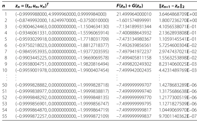
Table 1 Numerical results of Example 4.4 for iteration process (4.4)
n zn= (tn, un, vn)T F(zn) + G(zn) zn+1– zn2
1 (–0.9999988000, 4.9999960000, 0.9999984000) 21.499964000010 3.6464868709E+00 2 (–0.8749992000, 1.6249970000, –0.3750010000) –1.601574899991 1.8007236270E+00 3 (–0.9004624463, 0.0000000000, –1.1504634130) –7.134189931344 4.1056538071E–01 4 (–0.9346061331, 0.0000000000, –1.5596065914) –7.400888643932 2.1362893808E–01 5 (–0.9593029918, 0.0000000000, –1.7718031709) –7.473134980367 1.1059145541E–01 6 (–0.9750218023, 0.0000000000, –1.8812718377) –7.492639856561 5.7254600304E–02 7 (–0.9845953935, 0.0000000000, –1.9377203595) –7.497941972237 2.9747437021E–02 8 (–0.9903445225, 0.0000000000, –1.9669069578) –7.499405811158 1.5563253898E–02 9 (–0.9938004751, 0.0000000000, –1.9820816494) –7.499820249302 8.2314060025E–03 10 (–0.9959001978, 0.0000000000, –1.9900407454) –7.499942002435 4.4231489769E–03
. . .
. . .
. . .
. . .
50 (–0.9999828882, 0.0000000000, –1.9999828718) –7.499999999707 1.4278683289E–06 51 (–0.9999838977, 0.0000000000, –1.9999838817) –7.499999999740 1.3175686638E–06 52 (–0.9999848292, 0.0000000000, –1.9999848135) –7.499999999770 1.2177300519E–06 53 (–0.9999856901, 0.0000000000, –1.9999856747) –7.499999999795 1.1271827509E–06 54 (–0.9999864870, 0.0000000000, –1.9999864719) –7.499999999817 1.0449069970E–06 55 (–0.9999872257, 0.0000000000, –1.9999872109) –7.499999999837 9.7001140362E–07
We next provide the example as well as its numerical results.
Example . LetH=R. Minimize the following
-least square problem:
min
x∈Rx+
x
+ (, , )x– ,
wherex= (t,u,v)T.
LetF(x) =x+ (, , )x– andG(x) =x. Then∇F(x) = (t+ ,u+ ,v+ )T.
More-over,∇Fis -Lipschitz continuous and hence it is -inverse strongly monotone. From [] we know that, forr> ,
(I+r∂G)–(x)
=max|t|–r, sign(t),max|u|–r, sign(u),max|v|–r, sign(v)T.
Letzn= (tn,un,vn)T. Setf(x) =x and chooseαn=
–
n+,rn= ., anden=
(n+)(, , )T.
For the initial pointz= (t,u,v)T= (–, , )T, computing{zn}by the algorithm (.),
we obtain numerical results with an error –in Table .
From Table , we see thatz∞= (–, , –) is the minimizer ofF+Gand its minimum value is –..
Competing interests
The authors declare that they have no competing interests.
Authors’ contributions
All authors contributed equally to the writing of this paper. All authors read and approved the final manuscript.
Author details
1School of Science, University of Phayao, Phayao, 56000, Thailand.2Department of Mathematics, Faculty of Science,
Chiang Mai University, Chiang Mai, 50200, Thailand.
Acknowledgements
Received: 13 February 2015 Accepted: 17 June 2015
References
1. Lions, PL, Mercier, B: Splitting algorithms for the sum of two nonlinear operators. SIAM J. Numer. Anal.16, 964-979 (1979)
2. Passty, GB: Ergodic convergence to a zero of the sum of monotone operators in Hilbert space. J. Math. Anal. Appl.72, 383-390 (1979)
3. Brézis, H, Lions, PL: Produits infinis de resolvantes. Isr. J. Math.29, 329-345 (1978)
4. Güler, O: On the convergence of the proximal point algorithm for convex minimization. SIAM J. Control Optim.29, 403-419 (1991)
5. Martinet, B: Régularisation d’inéquations variationnelles par approximations successives. Rev. Fr. Inform. Rech. Oper.4, 154-158 (1970)
6. Rockafellar, RT: Monotone operators and the proximal point algorithm. SIAM J. Control Optim.14, 877-898 (1976) 7. Dunn, JC: Convexity, monotonicity, and gradient processes in Hilbert space. J. Math. Anal. Appl.53, 145-158 (1976) 8. Combettes, PL: Iterative construction of the resolvent of a sum of maximal monotone operators. J. Convex Anal.16,
727-748 (2009)
9. López, G, Martín-Márquez, V, Wang, F, Xu, HK: Forward-backward splitting methods for accretive operators in Banach spaces. Abstr. Appl. Anal.2012, Article ID 109236 (2012)
10. Takahashi, W: Viscosity approximation methods for resolvents of accretive operators in Banach spaces. J. Fixed Point Theory Appl.1, 135-147 (2007)
11. Wang, F, Cui, H: On the contraction-proximal point algorithms with multi-parameters. J. Glob. Optim.54, 485-491 (2012)
12. Xu, HK: A regularization method for the proximal point algorithm. J. Glob. Optim.36, 115-125 (2006)
13. Qin, X, Cho, SY, Wang, L: A regularization method for treating zero points of the sum of two monotone operators. Fixed Point Theory Appl.2014, 75 (2014)
14. Minty, GJ: On the maximal domain of a monotone function. Mich. Math. J.8, 135-137 (1961)
15. Nadezhkina, N, Takahashi, W: Weak convergence theorem by an extragradient method for nonexpansive mappings and monotone mappings. J. Optim. Theory Appl.128, 191-201 (2006)
16. Browder, FE: Nonexpansive nonlinear operators in a Banach space. Proc. Natl. Acad. Sci. USA54, 1041-1044 (1965) 17. Xu, HK: Iterative algorithms for nonlinear operators. J. Lond. Math. Soc.66, 240-256 (2002)
18. He, S, Yang, C: Solving the variational inequality problem defined on intersection of finite level sets. Abstr. Appl. Anal.
2013, Article ID 942315 (2013)
19. Baillon, JB, Haddad, G: Quelques proprietes des operateurs angle-bornes et cycliquement monotones. Isr. J. Math.26, 137-150 (1977)
20. Rockafellar, RT: On the maximal monotonicity of subdifferential mappings. Pac. J. Math.33, 209-216 (1970) 21. Hale, ET, Yin, W, Zhang, Y: A fixed-point continuation method for1-regularized minimization with applications to