Preconditioners for reduced saddle point systems arising in elliptic PDE constrained optimization problems

R E S E A R C H

Open Access

Preconditioners for reduced saddle point

systems arising in elliptic PDE-constrained

optimization problems

Yuping Zeng

_{, Siqing Wang, Hongru Xu and Shuilian Xie}

*_{Correspondence:}

[email protected] School of Mathematics, Jiaying University, Meizhou, 514015, China

Abstract

In this paper, we propose some preconditioning techniques for reduced saddle point systems arising from linear elliptic distributed optimal control problems. The

eigenvalues of preconditioned matrices are analyzed. Moreover, the bounds of these eigenvalues with respect to the mesh sizehare also obtained. Some numerical tests are presented to validate the theoretical analysis.

MSC: 65F10; 65F50

Keywords: PDE-constrained optimization; saddle point problem; preconditioning; eigenvalue estimate

1 Introduction

We consider the preconditioning techniques for solving the saddle point system arising from linear elliptic distributed optimal control problems:

min u,f

 u–uˆ



L₍₎+βf_L₍₎

subject to –u=f in,

u=g on∂, ()

where⊂Ris a simply connected polygonal domain with a connected boundary∂. The datauˆis the target function, and the parameterβis the Tikhonov regular parameter.u is the state variable, andf is called the control variable. Such problems are simple models, which were originally introduced by Lions in []. Some more complex formulations, which include control constraints or state constraints, can be found in [–].

For the elliptic PDE-constrained optimization problem (), we take the method based on discretize-then-optimize [] approach. More concretely, we use thePconforming finite elements for the approximations of the state variableuand the control variablef, which yields the following corresponding minimization problem [, ]:

⎧ ⎨ ⎩

min u,f

 u

T_{Mu– u}T_b+α+βfT_Mf

subject toKu=Mf+ d,

()

whereK∈Rm×m_{is the stiffness matrix,M∈R}m×m_{is the mass matrix. BothMandKare}

symmetric and positive definite. b∈Rm_{is the discrete Galerkin projection of the target}

functionuˆ.α=_ˆu

L₍₎, and d∈Rmcontains the terms arising from the boundaries of

finite element approximation of the stateu. Then, using the Lagrange multiplier technique for the minimization problem (), we can find that f, u andλsatisfy the following linear saddle point system []:

Ax= ⎛ ⎜ ⎝

βM  –M

 M K

–M K 

⎞ ⎟ ⎠

⎛ ⎜ ⎝ f u

λ

⎞ ⎟

⎠=

⎛ ⎜ ⎝  b

d ⎞ ⎟

⎠= g, ()

whereλis a vector of Lagrange multipliers. To obtain the above system, we have used the fact thatK=KT_{. Obviously, from the first equation of (), we can obtain that}

f= 

βλ. ()

Substituting () into (), we can easily obtain the following reduced system:

Ay=

M K

K –__βM u

λ

=

b

d

= g. ()

This paper is devoted to constructing efficient preconditioners for the reduced linear saddle point system (). Comparing with (), () is a smaller linear system so that it can help us to reduce computational cost. As we know, previous work has been mainly devoted to the development of efficient solution techniques for the original linear saddle point sys-tem (), such as the block diagonal preconditioner and the constraint preconditioner [], block triangular diagonal preconditioner [], diagonal and block-counter-tridiagonal preconditioning techniques []. Other recent work in this direction can also be found in [–]. For the reduced saddle point problem (), there have existed several pre-conditioning algorithms, we refer the reader to [–] for details. In our work, we extend similar preconditioning techniques, which were used in [, ] for system (), to the sad-dle point system (). We also refer the reader to [] for analogous discussions, where the optimal control of Stokes equations was addressed. The major contribution of our work is to establish the bounds of eigenvalues of the preconditioned matrices with respect to the discretization mesh sizeh, though we also provide the analysis of eigenvalues of the preconditioned matrices using the usual linear algebraic techniques developed in [, , ]. In particular, for the case that the Tikhonov parameterβis not very small, the bounds of eigenvalues of preconditioned matrices are proved to remain bounded away from  as h→ with a bound independent ofh. This suggests that they are optimal preconditioners in the sense that their performances are independent of the mesh sizeh.

2 Preconditioners for the Tikhonov parameter

β

When the Tikhonov parameterβis not very small, we may provide block-counter diago-nal preconditionerPbcdand block-counter-triangular diagonal preconditionerPbctdas the following form:

Pbcd=

 K

K 

()

and

Pbctd=

M K

K 

. ()

For the block-counter diagonal preconditionerPbcd, we have the following results.

Theorem . LetA∈Rm×mbe the coefficient matrix of the linear system()and Pbcd∈

Rm×m_{be defined in().Denote byν}

l the eigenvalue of K–M∈Rm×m,whereνl> ,l=

, , . . . ,m,and by x(l)_∈Cm_{the corresponding eigenvector for l= , , . . . ,m.Then} (i) the eigenvalues of the preconditioned matrixP–

bcdAare

λ(_kl)=  –

 βνle

(k+)πi

 _{, k= , ,l= , , . . . ,m,}

whereidenotes the imaginary unit;

(ii) the eigenvectors of the preconditioned matrixP–_bcdAare of the form

x(l) –

√

β μl e

(k+)πi

 K–Mx(l)

, l= , , . . . ,m,k= , .

Proof (i) By a direct calculation, we get

P–_ A=

 K–

K– 

M K

K –__βM

=

I –__βK–_M

K–_{M I}

. ()

To proceed, let

E=I–P_–A=

 __βK–_M

–K–_{M }

=

 __βD

–D 

, ()

whereD=K–_{M. Therefore,}

E=

–__βD _  –__βD

. ()

Then from () we can know that ifνlis the eigenvalue ofK–M, then the eigenvalues

ofEare

 βνle

(k+)πi

 _{,k= , . Thus, the eigenvalues of the preconditioned matrixP}–

bcdA

are  –

 βνle

(k+)πi

(ii) By similar techniques used in the proof of (ii) in Theorem ., we can obtain the

corresponding conclusions.

For the block-counter-triangular diagonal preconditionerPbctd, we have the following results.

Theorem . LetA∈Rm×mbe the coefficient matrix of the linear system()and Pbctd∈

Rm×m_{be defined in().Denote byν}

lthe eigenvalue of K–M∈Rm×m,whereνl> ,l=

, , . . . ,m,and by y(l)_∈Cm_{the eigenvector of(K}–_M)_{for l= , , . . . ,m.Then}

(i) the eigenvalues of the preconditioned matrixP_bctd– Aarewith algebraic multiplicity m,and the remaining eigenvalues equal __βν_l+ ,l= , , . . . ,m;

(ii) the eigenvectors of the preconditioned matrixP–

bctdAare of the form

x 

, ∀x∈Cm\{}, and

–_νK–My(l) y(l)

, l= , , . . . ,m.

Proof (i) A straightforward calculation shows that

P–_bctdA=

 K–

K– –K–MK–

M K

K –__βM

=

I –__βK–M  I+__βK–MK–M

. ()

It follows from the above equality that the eigenvalues of the preconditioned matrixP– bctdA are  with algebraic multiplicitym, andmeigenvalues with the form  + 

βν

_{, whereνis}

any eigenvalue of the matrixK–_{M. This demonstrates the conclusions of (i).} (ii) Let{λ, (x,y)T_{}be an eigenpair for the matrixP}–

bctdA, then from the expression of P–_bctdAin (), we have

I –

βK

–_M

 I+__βK–MK–M x y

=

x y

=λe,

or the above equation can be rewritten as ⎧

⎨ ⎩

(x–__βK–_{My) =λx,}

(I+__βK–MK–M)y=λy.

It is easy to see that ifλ= , theny= , thus the corresponding eigenvectors take the form

e=

x 

, with∀x∈Cm\{}. ()

Ifλ= , we have

x= 

β( –λ)K

–_{My ()}

and

Thus,λ=__βν_{+ , withνan eigenvalue of the matrixK}–_{M. Direct computations lead to}

x= –

νK

–_{My. ()}

Obviously,y∈Cm_{is an eigenvector of the matrix (K}–_M)_{. This completes the proof.} Furthermore, using the theory of finite element methods, we can use the results stated in the above two theorems to obtain more concrete bounds that involved the discretiza-tion mesh sizeh. Since in our numerical tests we use theP conforming finite elements to discretize problem (), we recall the following lemma from [, ] which will be used frequently in our theory analysis.

Lemma . LetTh={Ti:i= , , . . . ,Eh}be a family of quasi-uniform and shape regularity

triangulations of the domain⊂R_{.Denote by h}

Ti the diameter of the element Tiand h=maxTi∈ThhTi.For the Pconforming finite element,the mass matrix M and the stiffness matrix K satisfy

ch≤x

T_Mx

xT_x ≤ch

_{, ()}

dh≤x

T_Kx

xT_x ≤d, ()

∀x= ∈Rm_{.Constants c}

,c,dand dare positive and independent of h andβ.

With the above prepared techniques, we can obtain the following two corollaries.

Corollary . Letλbe an eigenvalue of P–

bcdA,with PbcdandAbeing defined in()and(). Then the following bound holds:

 + c

 h

βd_ ≤ |λ| ≤

 + c  

βd_. ()

Proof From (i) in Theorem ., the eigenvalues ofP– bcdAare

λ(_kl)=  –

 βνle

(k+)πi

 _{, k= , ,l= , , . . . ,m.}

A direct calculation shows that

λ(_kl)=  +  βν



l – 

 βcos

(k+ )π

 =  +

 βν



l. ()

In the last step of the above equation we have used the fact thatcos(k+)π

 = .

Thus, from the above equality, we know that if we want to bound|λ(_kl)|, it is sufficient to boundνl. Recalling thatνlis an eigenvalue ofK–M, we get

K–Mx=νlx,

thus xTMx=νlxTKx,

νl=

xT_Mx

xT_Kx. ()

From () in Lemma ., we obtain

 d ≤

xT_x

xT_Kx≤



dh. ()

Thus, from (), () and () we get

ch d ≤νl≤

c

d. ()

Then the corollary follows by () and ().

Corollary . Letλbe an eigenvalue of P–

bctdA,with PbctdandAdefined in()and(). Then the eigenvalues of the preconditioned matrix P–

bctdAarewith algebraic multiplicity m,the remaining m eigenvalues can be bounded as follows:

 + c

 h βd_ ≤λ≤

 + c

 

βd_. ()

Proof From (i) in Theorem ., using the same proof procedure as in Corollary ., we

can obtain the corresponding conclusion.

Remark . From () and () in Corollaries . and ., we can see that the eigenvalues

of the preconditioned matricesP–

bcdAandP–bctdAsatisfy

≤ |λ| ≤

 + c

 

βd_ ash→. ()

Furthermore, ifβ is not too small, then from () we know that the eigenvalues of the preconditioned matricesP–

bcdAandP–bctdAare clustered. When the parameterβ is not too small, () also means thatPbcdandPbtcdmay perform as optimal preconditioners in the sense that their performances are independent of the mesh sizeh.

Remark . In practical computations, we may choose good approximationsK˜andM˜ for KandM, respectively. Then the corresponding preconditionersPbcdandPbctdare replaced by

˜

Pbcd=

 K˜

˜

K 

and Pbctd˜ =

˜

M K˜

˜

K 

,

3 Preconditioners for the Tikhonov parameter

β

In this section, we discuss block diagonal and block-triangular diagonal preconditioning techniques for the linear system () and analyze the eigenvalues and eigenvectors of the preconditioned matrices. The block diagonal preconditioner is given by

Pbd=

M 

 –__βM

, ()

and the block-triangular diagonal preconditioner is of the form

Pbtd=

M K

 –__βM

. ()

Moreover, we find that both the preconditioned matricesP–

bdAandP–btdAhave eigenvalues around  when the Tikhonov parameterβ is sufficiently small (i.e.,β). These prop-erties are stated in the following two theorems. The spectral analysis for preconditioned matrices is largely based on the references [, ]. First, we consider the block diagonal preconditioner.

Theorem . LetA∈Rm×m_{be the coefficient matrix of the linear system()and Pbd∈} Rm×m_{be defined in().Setμ}

lthe eigenvalue M–K∈Rm×m,whereμl> ,l= , , . . . ,m,

and x(l)∈Cmthe corresponding eigenvector for l= , , . . . ,m.Then

(i) the eigenvalues of the preconditioned matrixP– bdAare

λ(_kl)=  –βμle (k+)πi

 _{, k= , ,l= , , . . . ,m,}

whereidenotes the imaginary unit;

(ii) the eigenvectors of the preconditioned matrixP–

bdAare of the form

⎛

⎝–



√

βμle

(k+)πi



M–Kx(l)

x(l)

⎞

⎠, l= , , . . . ,m,k= , .

Proof (i) A simple calculation shows that

P–_bdA=

M– _

 –βM–

M K

K –__βM

=

I M–_K

–βM–_{K I}

. ()

To proceed, let

C=I–P–_bdA=

 –M–_K

βM–_{K }

=

 –B

βB 

, ()

whereB=M–_{K. Therefore,}

C=

–βB _  –βB

From () we can know that ifμlis the eigenvalue ofM–K, then the eigenvalues ofC

are√βμle (k+)πi

 ,k= , . Thus, the eigenvalues of the preconditioned matrixP–

bdAare  –√βμle

(k+)πi

 _{,k= , . This leads to (i).}

(ii) Letμlbe the eigenvalue ofM–K∈Rm×mandx(l)∈Cmbe the corresponding

eigen-vector forl= , , . . . ,m, then

M–KM–Kx(l)=μ_lx(l).

Multiplying both sides of the above equation by –βyields

–βM–KM–Kx(l)= –βμ_lx(l)=βμle (k+)πi

 _x(l)_,

i.e.,

–βM–K_√  βμle

(k+)πi



·M–Kx(l)=βμle (k+)πi

 _x(l)_{. ()}

Let

y= –_√ 

βμle (k+)πi



M–Kx(l),

then

–M–Kx(l)=βμle (k+)πi

 _{y. ()}

From the expressions of () and () we obtain

⎧ ⎨ ⎩

–Bx(l)_{= (}√_βμ

le (k+)πi

 )y,

βBy= (√βμle (k+)πi

 _)x(l)_.

Thus,

C

y x(l)

=

 –B

βB  y x(l)

=βμle (k+)πi



y x(l)

.

Therefore, ifx(l)_∈Cm_{is an eigenvector of the matrixB, then}y x(l)

is the eigenvector of the

matrixC∈Rm×m. This finishes the proof.

Then we turn our attention to the block-triangular diagonal preconditioner.

Theorem . Let A∈Rm×m _{be the coefficient matrix of the linear system () and}

Pbtd∈Rm×m be defined in().Set μlthe eigenvalue of M–K∈Rm×m,whereμl> ,

l= , , . . . ,m,and x(l)_∈Cm_{the eigenvector of the matrix(M}–_K)_{for l= , , . . . ,m.Then}

(i) the eigenvalues of the preconditioned matrixP–

(ii) the eigenvectors of the preconditioned matrixP–

btdAare of the form

 y

, ∀y∈Cm\{}, and

x(l) –_μM–Kx(l)

, l= , , . . . ,m.

Proof (i) By a direct calculation we get that

P–_btdA=

M– _βM–_KM–

 –βM–

M K

K –__βM

=

I+ βM–_KM–_{K } –βM–_{K I}

. ()

It follows from the above equality that the eigenvalues of the preconditioned matrix P–_btdAare  with algebraic multiplicitym, andmeigenvalues with the form  + βμ_{, where}

μis any eigenvalue of the matrixM–_{K. This demonstrates the conclusions of (i).} (ii) Let{λ, (x,y)T_{}be an eigenpair for the matrixP}–

btdA, then from the expression ofP–btdA in (), we have

I+ βM–_KM–_{K } –βM–K I

x y

=λ

x y

=λe,

or the above equation can be rewritten as ⎧

⎨ ⎩

(I+ βM–KM–K)x=λx,

–βM–_Kx+y=λy.

It is easy to see that ifλ= , thenx= , thus the corresponding eigenvectors take the form

e=

 y

, with∀y∈Cm\{}. ()

Ifλ= , we have

y= β  –λM

–_{Kx ()}

and

I+ βM–_KM–_{Kx=λx. ()}

Thus,λ= βμ_{+ , withμan eigenvalue of the matrixM}–_{K. A direct calculation shows} that

y= –

μM

–_{Kx. ()}

Corollary . Letλbe an eigenvalue of P–

bdA,with Pbd andAdefined in()and(). Then the following bound holds:

 +βd

  c



≤ |λ| ≤

 +βd

  c

h

. ()

Proof From (i) in Theorem ., the eigenvalues ofP– bdAare

λ(_kl)=  –βμle (k+)πi

 _{, k= , ,l= , , . . . ,m.}

A direct calculation leads to

λ(_kl)=  + βμ_l – βcos(k+ )π

 =  + βμ 

l. ()

In the last step of the above equation we have used the fact thatcos(k+)_ π = .

Thus, from the above equation, we know that if we want to bound|λ(_kl)|, it is enough to boundμl. Recalling thatμlis an eigenvalue ofM–K, we get

M–Kx=μlx,

i.e.,Kx=μlMx,

thus xTKx=μlxTMx,

μl=

xT_Kx

xT_Mx. ()

From () in Lemma ., we obtain

 ch ≤

xT_x

xT_Mx≤



ch. ()

Thus, from (), () and () we get

d c

≤μl≤

d ch

. ()

Then the corollary follows by () and ().

Corollary . Letλbe an eigenvalue of P–_btdA,with Pbtd andAdefined in()and(). Then the eigenvalues of the preconditioned matrix P–

btdAarewith algebraic multiplicity m,the remaining m eigenvalues can be bounded as follows:

 +βd

  c



≤λ≤

 +βd

  c

h

. ()

Proof From (i) in Theorem ., using the same proof procedure as in Corollary ., we

Remark . From Theorems . and ., we can see that the eigenvalues of the precon-ditioned matricesP–

bdAandP–btdAare around  when the Tikhonov parameterβis suffi-ciently small.

Remark . In actual computations, we may choose good approximationsK˜ andM˜ for KandM, respectively. Then the corresponding preconditionersPbdandPbtdare replaced by

˜

Pbd=

˜

M 

 –__βM˜

and Pbtd˜ =

˜

M K˜

 –__βM˜

,

respectively. Some examples of properM˜ andK˜ were presented in [, ].

4 Numerical experiments

The test problem we consider is the following linear elliptic optimal control problem:

min u,f

 u–uˆ



+βf subject to –u=f in,

u=  on∂,

where= (, )×(, ),uˆ∈L_{() is given by}

ˆ

u= ⎧ ⎨ ⎩

 if (x,y)∈[,_]_, , otherwise.

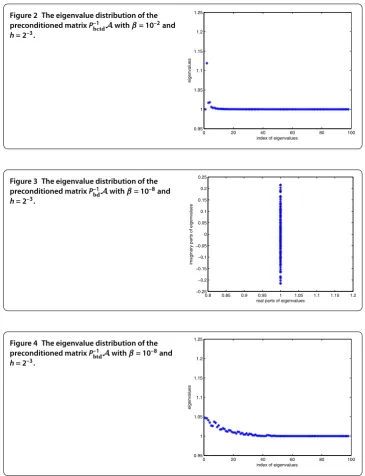
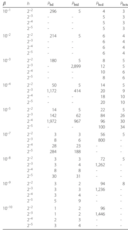
Our numerical experiments are performed by MATLAB. We consider four uniformly refined meshes, which are constructed by subsequently splitting each triangle into four triangles by connecting the midpoints of the edges of the triangle. First, by setting the regular parameterβ= – _{(not very small), we show the eigenvalues of the} precondi-tioned matricesP–_bcdAandP–_bctdAin Figures  and , they are both clustered. These results demonstrate the theoretical analysis in Theorems . and .. Also, by setting the regular parameterβ= –(very small), we show the eigenvalues of the preconditioned matrices

Figure 2 The eigenvalue distribution of the preconditioned matrixP–1

bctdAwithβ= 10–2and h= 2–3_.

Figure 3 The eigenvalue distribution of the preconditioned matrixP–1

bdAwithβ= 10

–8_and

h= 2–3_.

Figure 4 The eigenvalue distribution of the preconditioned matrixP–1_btdAwithβ= 10–8and h= 2–3.

P–

bdAandP–btdAin Figures  and , both of them are clustered. These results validate the theoretical analysis in Theorems . and ..

Furthermore, for comparison, we show the number of iterations for different precondi-tioners with different regular parameters in Table . In all implementations, we use zero as initial guess and stop the iteration whenr(k)_(=b–Ax(k)₎

Table 1 The number of iterations for different preconditioners

β h Pbd Pbtd Pbcd Pbctd

10–1 2–2 296 5 4 3

2–3 - - 5 3

2–4 - - 5 3

2–5 - - 5 3

10–2 ₂–2 _{214 5 6 4}

2–3 _{- - 6 4}

2–4 _{- - 6 4}

2–5 _{- - 6 4}

10–3 ₂–2 _{180 5 8 5}

2–3 _{- 2,899 12 5}

2–4 _{- - 10 6}

2–5 _{- - 8 6}

10–4 ₂–2 _{50 5 14 5}

2–3 _{1,172 414 20 9}

2–4 _{- - 18 10}

2–5 _{- - 20 10}

10–5 ₂–2 _{14 5 22 5}

2–3 142 62 84 26

2–4 1,972 967 96 30

2–5 - - 100 34

10–7 ₂–2 _{3 3 56 5}

2–3 _{8 6 800}

-2–4 _{28 23 -}

-2–5 _{284 188 -}

-10–8 ₂–2 _{3 3 72 5}

2–3 _{3 4 1,262}

-2–4 _{8 8 -}

-2–5 _{30 31 -}

-10–9 ₂–2 _{3 2 94 8}

2–3 _{3 3 1,236}

-2–4 _{3 4 -}

-2–5 _{5 9 -}

-10–10 ₂–2 _{1 2 96}

-2–3 1 2 1,446

-2–4 2 3 -

-2–5 3 4 -

-regular parameterβis very small, the number of iterations ofPbdandPbtdpreconditioners is smaller thanPbcdandPbctd, thusPbdorPbtdpreconditioners are our choices.

Competing interests

The authors declare that they have no competing interests.

Authors’ contributions

The main idea of this paper was proposed by YZ. All authors contributed equally in writing this article and read and approved the final manuscript.

Acknowledgements

We thank the anonymous referees for their valuable comments and suggestions which led to an improved presentation of this paper. This work was supported by the opening fund of Jiangsu Key Lab for NSLSCS (Grant No. 201402), the Training Program for Outstanding Young Teachers in Guangdong Province (Grant No. 20140202), and the Educational Commission of Guangdong Province (Grant No. 2014KQNCX210).

Received: 30 March 2015 Accepted: 22 October 2015 References

2. Bergounioux, M, Ito, K, Kunisch, K: Primal-dual strategy for constrained optimal control problems. SIAM J. Control Optim.37, 1176-1194 (1999)

3. Bergounioux, M, Kunisch, K: Primal-dual strategy for state-constrained optimal control problems. Comput. Optim. Appl.22, 193-224 (2002)

4. Casas, E: Control of an elliptic problem with pointwise state constraints. SIAM J. Control Optim.31, 1297-1327 (1993) 5. Rees, T, Dollar, HS, Wathen, AJ: Optimal solvers for PDE-constrained optimization. SIAM J. Sci. Comput.32, 271-298

(2010)

6. Bai, Z: Block preconditioners for elliptic PDE-constrained problems. Computing91, 379-395 (2011)

7. Rees, T, Stoll, M: Block-triangular preconditioners for PDE-constrained optimization. Numer. Linear Algebra Appl.17, 977-996 (2010)

8. Herzog, R, Sachs, E: Preconditioned conjugate gradient method for optimal control problems with control and state constraints. SIAM J. Matrix Anal. Appl.31, 2291-2317 (2010)

9. Pearson, JW, Wathen, A: A new approximation of the Schur complement in preconditioners for PDE-constrained optimization. Numer. Linear Algebra Appl.19, 816-829 (2012)

10. Schöberl, J, Zulehner, W: Symmetric indefinite preconditioners for saddle point problems with applications to PDE-constrained optimization problems. SIAM J. Matrix Anal. Appl.29, 752-773 (2007)

11. Zhang, G, Zheng, Z: Block-symmetric and block-lower-triangular preconditioner PDE-constrained optimization problems. J. Comput. Math.31, 370-381 (2013)

12. Bai, Z, Benzi, M, Chen, F, Wang, Z: Preconditioned MHSS iteration methods for a class of block two-by-two linear systems with applications to distributed control problems. IMA J. Numer. Anal.33, 343-369 (2013)

13. Borzì, A, Schulz, V: Multigrid methods for PDE optimization. SIAM Rev.51, 361-395 (2009)

14. Lass, O, Vallejos, M, Borzi, A, Douglas, CC: Implementation and analysis of multigrid schemes with finite elements for elliptic optimal control problems. Computing84, 27-48 (2009)

15. Schöberl, J, Simon, R, Zulehner, W: A robust multigrid method for elliptic optimal control problems. SIAM J. Numer. Anal.49, 1482-1503 (2011)

16. Simoncini, V: Reduced order solution of structured linear systems arising in certain PDE-constrained optimization problems. Comput. Optim. Appl.53, 591-617 (2012)

17. Vallejos, M, Borzì, A: Multigrid optimization methods for linear and bilinear elliptic optimal control problems. Computing82, 31-52 (2008)

18. Zulehner, W: Nonstandard norms and robust estimates for saddle point problems. SIAM J. Matrix Anal. Appl.32, 536-560 (2011)

19. Wang, S: A class of preconditioned iterative methods for the optimal control of the Stokes equations. Master thesis, Nanjing normal university (May 2014)