One Market, One Money, One Price?
Allington, Nigel FB and Kattuman, Paul A and Waldmann,
Florian A
21 March 2005
Online at
https://mpra.ub.uni-muenchen.de/835/
Nigel F.B. Allington,a Paul A. Kattuman,b and Florian A. Waldmannc
aGonville and Caius College, University of Cambridge,
and Cardiff University
bJudge Business School and Corpus Christi College,
University of Cambridge
cCitigroup Global Markets, London and Wolfson College,
University of Cambridge
The introduction of the euro was intended to integrate mar-kets within Europe further, after the implementation of the 1992 Single Market Project. We examine the extent to which this objective has been achieved, by examining the degree of price dispersion between countries in the euro zone, compared to a control group of EU countries outside the euro zone. We also establish the role of exchange rate risk in hampering ar-bitrage by estimating the euro effect for subgroups within the euro zone, utilizing differences among EU countries in partici-pation in the Exchange Rate Mechanism. Our results, in con-trast with previous empirical research, suggest robustly that the euro has had a significant integrating effect.
JEL Codes: E31, E42, F01.
Over the past two decades, markets within the European Union (EU) have become progressively more integrated as internal barri-ers to trade have been dismantled. Two crucial steps in this process were the completion of the Single Market Project in 1992 and the start of Economic and Monetary Union (EMU) in 1999. The first removed the remaining physical, administrative, and technical bar-riers to integration and stimulated competition. The second intro-duced a common currency and eliminated exchange rate variations
∗We are grateful to Eurostat for providing the data analyzed in this paper. Eurostat bears no responsibility for the analysis and conclusions reported here. We should like to thank an anonymous referee for comments on an earlier ver-sion, but remain responsible for any errors or omissions. Corresponding author: Kattuman, e-mail: p.kattuman@jbs.cam.ac.uk.
between the eleven (later twelve) members of the euro zone.1 In the
widely quoted and influential report “One Market, One Money,” the European Commission (1990) argued that “without a completely transparent and sure rule of the law of one price for tradable goods and services, which only a single currency can provide, the sin-gle market cannot be expected to yield its full benefits—static and dynamic.” The single currency would deepen integration by lower-ing exchange-rate-risk premia, lower uncertainty, make cross-border business much more profitable, and lower transaction costs, thereby saving the equivalent of approximately 1 percent of EU15 GDP.
This viewpoint was reiterated in the 1996 review of the single market: “increased price transparency will enhance competition and whet consumer appetites for foreign goods; price discrimination be-tween different national markets (in the EU) will be reduced” (Euro-pean Commission 1996). When the euro actually became an account-ing reality in 1999, the European Commission (1999) anticipated that it would “squeeze price dispersion in EU markets.”
The recent publication of a newly revised, consistent, and com-prehensive data set on price indices for the period from 1995 has made it possible to undertake a detailed analysis of price convergence within the EU. We test the hypothesis that greater market integra-tion, followed by a common currency, has rendered the Law of One Price (LOOP) valid for the EU. Our results robustly suggest that the euro has had a positive effect on price convergence for tradable goods, among EMU members relative to non-EMU members, over and above a general EU-wide tendency towards price convergence. It is also evident that risk, due to volatility of nominal exchange rates prior to the introduction of EMU, has had a significant bearing on the process of price convergence.
The structure of this paper is as follows. An overview of the rel-evant theory and the empirical literature is provided in section 1, including the benefits derived from a single currency. Section 2 describes the data and section 3 discusses the methodology used. Section 4 reports the results of our analysis. Conclusions are offered in section 5.
1The 1999 members were Austria, Belgium, Finland, France, Germany,
1. Theory and Literature
1.1 Theory
In the international economics literature, the LOOP and its aggre-gate counterpart, Purchasing Power Parity (PPP), have provided a useful benchmark for the dynamics of relative prices. The Law of One Price states that prices of identical tradable goods priced in the same currency should, under competitive conditions, be equal across all locations, national and international. If prices differ, then arbitrageurs, subject to certain threshold effects, would profit from buying the goods where they are comparatively cheap and selling them where they are comparatively expensive. The price of nontrad-able goods, normally excluded from the LOOP analysis, can also be expected to converge, with a sufficiently high degree of economic integration.
From a theoretical point of view, the failure of LOOP, and hence of PPP, has several explanations. In a common market like the EU, where tariffs, trade quotas, and other informal barriers have been removed, one obvious reason that remains would be transport costs. Shipping costs permit price differentials between more distant mar-kets without encouraging arbitrage. In a seminal article, Engel and Rogers (1996) found that distance, as a convenient control for trans-port costs, explains relative price dispersion across ten U.S. and nine Canadian cities; this result has been confirmed by Parsley and Wei (1996 and 2001), Cecchetti, Nelson, and Sonora (1999), and more re-cently by Haskel and Wolf (2001). Engel and Rogers also reveal that the border effect is more decisive than distance, even when both countries share the same language and similar cultural and politi-cal traditions. They speculate that the EU could also be affected by similar border effects, and Beck and Weber (2003) report evidence for this.
across Europe will not be surprising. Technological advances such as Internet price search engines should erode these information barriers over time, but Baye et al. (forthcoming)—analyzing prices of a selec-tion of homogenous goods sold via Internet price listing services— found that, in fact, price dispersion within EMU countries increased, relative to price dispersion within non-EMU countries, after the introduction of the euro.
Another explanation suggests that highly traded goods contain significant nontraded components and this frustrates price conver-gence (Rogoff 1996). Consumer prices include the price of the prod-uct itself, but also imputed rents, shipping costs, labor costs, and insurance premiums from nontraded goods. These cost factors may affect the prices of nontraded intermediate goods and thereby have an impact on the degree of price dispersion for traded final goods.
Exchange rate risk can also raise costs of cross-country arbitrage. An arbitrageur buying high-priced products in, say, Sweden, with the intention of selling them in the United Kingdom, faces the risk that profits are eliminated through exchange rate movements before the goods have been sold. The risk would be higher if long-term investments are necessary for seizing potential arbitrage opportuni-ties, because exchange rate hedges with maturity dates longer than one year are hard to obtain (HM Treasury 2003). Price dispersion between homogeneous tradable goods could arise due to transac-tion costs involved in cross-border payment, currency conversion, or settlement delay.
Finally, arbitrage by consumers might be hampered by the lack of price transparency. Although comparisons of prices between coun-tries need only basic calculations, the psychological effect of using a different yardstick could be large and potentially inhibiting. Money illusion cannot be ruled out, according to Fehr and Tyran (2001), but whether this applies in a single-currency context is debatable.
1.1.1 The Benefits of a Common Currency
controversial papers, Rose (2000, 2002) and jointly with van Wincoop (2001) and Glick (2001) established that countries with the same currency traded with each other twice as much as those with
dif-ferent currencies.2 And Micco, Stein, and Ordo˜nez (2003) provided
evidence that the introduction of the euro increased trade among the members of the single currency and also those that remained outside, although the 8–16 percent increase in volume terms falls way short
of the estimates of Rose.3
Beck and Weber (2003) attributed the failure of the LOOP to ex-change rate volatility that impedes price convergence, and Goldberg and Verboven (2004) demonstrated that such volatility contributed significantly to price dispersion in the European car market. But they argued that the EU could facilitate price convergence for cars by removing restrictions on competition that had previously been sanctioned by the European Commission as a concession to man-ufacturers. The threat of new entrants into the domestic market and hence greater competition would put downward pressure on producers’ prices (Freeman 1995).
Price convergence could also be stimulated by a common mon-etary policy and more particularly in the nontraded goods sector
through the Balassa-Samuelson hypothesis (1964).4 Furthermore,
Eleftheriou (2003) found that euro-zone countries (including Greece, Portugal, and Spain) for which the common interest rate was inap-propriately low, were also poorer countries with low relative price levels. A low common interest rate led to an above-EMU average inflation rate (“catch-up inflation”) in these countries and thus to price convergence. The predictive power of the common interest rate in terms of future inflation rates has proved to be surprisingly robust (Honohan and Lane 2003).
The EMU has the potential to remove exchange rate risk, trans-action costs, and the veil over price transparency. While price
2The relationship between market integration and the volume of trade would
not be monotonic.
3Rose’s results have been challenged by, among others, Persson (2001) and
M´elitz (2001).
4Converging and higher productivity levels in the traded goods sector may
convergence will be stimulated, price dispersion will remain to a greater or lesser degree. United States’ price convergence has been used as a predictor for the EU, given their similar size, structure, and culture, although the EU has more languages. Begg et al. (2001) found substantially lower price dispersion in the United States than in the EU and concluded that the potential for price convergence in
the EU remained large (but see Math¨a 2003; Rogers 2001 and 2002).
1.2 Empirical Evidence
Sifting the evidence on price convergence p and post-EMU re-quires a great deal of care. This stems from the different method-ologies employed by researchers as well as empirical issues such as differences in data sources; whether countries or cities, or single com-modities or multiproduct groups, are the focus, and whether appro-priate controls were used. In practice, data quality and availability frame the hypothesis that can be tested. The results from previous research that encompasses EMU have been summarized in table 1 in the appendix and these are assessed below. Eleven studies offer the most germane comparison with our own work, two of which found a positive euro effect, five a mixed euro effect, and four a negative or no euro effect.
1.2.1 Positive or Mixed Euro Effect
National borders prevent prices from converging as Rose (2002) and others have shown. Extending that analysis, Beck and Weber (2003) in their study of eighty-one cities and ten categories of goods over the period 1991–2002 found that crossing a border was equivalent to adding seventy-four miles to the distance between cities. That was a much lower figure than previous researchers had found, and—of greater significance—they report that intranational price dispersion fell by 80 percent after the introduction of the euro. Isgut (2002) an-alyzed two balanced panels of 116 cities and 69 goods and 79 cities and 123 goods in 2001 and concluded that the same currency reduces price differences generally by 2–3 percent (using standard deviations of log price differences across city pairs) and in the EMU specifi-cally, by 5 percent, even when EU had been controlled for. Friberg
introduction of the euro using data on ninety-two supermarket prod-ucts sold in Luxembourg and four contiguous regions, taking into account psychological pricing (pricing just below a round number of euros, typically ending 0.95 or 0.75) and found greater convergence in psychological prices than in fractional prices.
Five studies found mixed results. In an extensive analysis of eighty-three cities and ninety-five commodities over the period 1990– 2000, Parsley and Wei (2001) found 4.3 percent lower price dispersion following EMU and that the Belgium-Luxembourg currency union had 8 percent lower price dispersion. They estimate that this result equates to a drop in tariffs of 4 percent (the effect of any currency union is one order of magnitude more important than the fall in ex-change rate volatility). But once EU membership is controlled for, the EMU effect is no longer found to be significant. In a more re-stricted analysis of economic regions contiguous with Luxembourg,
Math¨a (2003) examined ninety-two supermarket products at four
dates in 2001 and 2002 and showed that monetary union led to price convergence, except that as distance increased, prices rose by 0.025 percent. However, the products were sold at different supermarkets and might not be strictly comparable. He predicted that the smaller distances across Europe in comparison with the United States indi-cate that price convergence in the EU has much further to go.
Lutz (2004) compared the long-standing Belgium-Luxembourg currency union with the rest of the EU to determine whether the currency union had generated higher levels of price convergence for ninety car models over the period 1993–98. He reports a 4 percent lower price differential within the currency union even when the other determinants of economic integration had been controlled. In an earlier study, Lutz (2003) had included a smaller sample of cars
(seventeen models), but also The Economist magazine, Big MacsR,
and data on thirteen categories of goods collected by UBS over a thirty-year period ending in 2000. He had only one post-EMU date to measure any euro effect on a small commodity sample. Price
conver-gence could be found forThe Economist, but no significant euro effect
this convergence had occurred before the introduction of the single currency.
1.2.2 Negative or No Euro Effect
A number of macroeconomic studies have looked at the impact of the Single Market Project on price convergence. Rogers (2002) found that most of the convergence (in his study of 139 commodities in twenty-five EU cities) occurred before 1994, with the EU level close to that found in the United States. Of more relevance to us is his study with Engel (2004) that assessed 101 narrowly defined tradable goods and 38 nontraded goods in eighteen cities in eleven EU countries, using seven non-EU countries as a control, over the period 1990–2002/3. They confirm the earlier result, but now found that the price dispersion for tradables had somewhat perversely in-creased after EMU and that the result applied to those countries outside the euro zone as well as to those inside the zone.
In a microeconomic study of 150 car models in five EU countries (one non-EMU) over the period 1970–2000, Goldberg and Verboven (2004) report converging prices between 1990 and 1992, but diver-gence thereafter, specifically in the United Kingdom and in Italy. Fi-nally, in the first study of Internet prices, Baye et al. (forthcoming) collected the weekly prices of twenty-eight mostly electronic prod-ucts during 2001 and 2002 from a price comparison site (Kelkoo) for seven countries, including four in the euro zone. Although the EU had lower price dispersion than the United States for compara-ble goods, by 2002 the goods were priced 10 percent higher in the euro-zone countries than they were in the non-euro-zone ones.
1.2.3 Relevance of the Findings
unrepresentative of the whole country. This criticism affects many of the studies, including Parsley and Wei (2001), Beck and Weber (2003), and Engel and Rogers (2004). In testing LOOP, it is unsat-isfactory that unit value studies cannot use identical commodities, or product categories that are standardized. Quality differences can
bias results. The results from single products such asThe Economist
or Big MacsR, while interesting, are too limited to be generalizable.
This paper employs a consistent series of country-level compar-ative price indices for a large number of product groups. Unlike most of the other studies, it includes four post-EMU date points. We find that the earlier harmonization effect from economic integra-tion and the macroeconomic policy convergence effect had not been fully played out in the run up to the euro, and that there was a significant euro effect.
2. Data
2.1 Data Description
2.1.1 Data Collection and Categorization
The data used for our empirical analysis were provided by Eurostat. The data contain comparative price level (CPL) indices for individual
consumption expenditure5 in 200 product groups for the fifteen EU
countries over the period 1995–2002.6 The group categorization
fol-lows the United Nations “Classification of Individual Consumption
According to Purpose.”7 The data were published on December 18,
2003, based on the European System of Accounts, 1995 (ESA95)
reg-ulation revision.8 This is the most disaggregated level at which data
is currently held by Eurostat. The revision makes the data compa-rable across the period 1995–2002, whereas previously this was only
possible for either the period pre-1999or post-1999.
5Retail prices including VAT.
6Eurostat uses the term “comparative price level” rather than relative price
level to signify that price levels are comparable between countries at a defined level of aggregation.
7For details, see United Nations Statistics Division, http://unstats.un.org/
unsd/cr/family2.asp?Cl=5.
8Commission Regulation (EC) 2223/1996 of June 25, 1996; see Eurostat
The prices of consumer goods and services are collected by Eu-rostat in cooperation with the national statistical agencies for the Eurostat-OECD comparison program every three years. Data are gathered for all goods and services at six collection dates, one every half year (using a rolling benchmark approach). Prices in between the three-year collections are extrapolated with the respective monthly consumer price index. The data are used to construct a PPP series for the products, i.e., ratios of prices denoted in respective currencies. The notion of comparing “identical” products is constrained by consumption patterns in the relevant countries. For example, a mainstream product sold in supermarkets with a low retail price in Germany might only exist as a niche product with a high retail price in the United Kingdom. Eurostat attempts to ensure that the se-lected products are commonly found in as many participating coun-tries as possible, but they do not necessarily have to be available in all the countries (Eurostat 2003b).
Among the 200 product groups, 39 are so-called reference PPPs, for which no data are collected directly (e.g., services of general prac-titioners, heat energy, and life insurance). Their value is imputed en-tirely from other included product groups, and so they are excluded from our analysis. The scope of our analysis is given in table 2 in the appendix. The data allow a distinction between tradables and nontradables, shown in the column labeled “Category.” From the 161 product groups with good quality data, 115 tradable products can be identified. Nontradables are categorized into low and high sunk-cost products in order to test the hypothesis that low sunk-cost products may converge faster due to lower barriers for arbitrage. Tradables can likewise be separated into broader categories of product groups, which are less or more tradable (e.g., perishable and nonperishable foods). The distinction is shown in table 3 in the appendix.
Greece has been excluded from the analysis, because it did not join the EMU in 1999 and treating it as a non-EMU member would bias the non-EMU group for 2001 and 2002.
2.1.2 Computations of the Comparative Price Level Series
rate that would be necessary to equalize price levels between two countries. The aggregation of the PPP series produces a set of PPP
exchange rates relative to the EU average.9 The annual CPL indices
are computed as a ratio of the respective PPP exchange rate over
the annual average of the respective nominal exchange rate, e, as
shown in equation (1) for countryc:
CP Lc/EU =
P P Pc/EU
ec/EU ·100 (1)
The CPL series can be used to test whether PPP holds, in which case the CPL equals 100, i.e., the ratio of the price levels equals the nominal exchange rate. Thus, deviations of a country’s CPL index from the EU average (that always equals 100) provide information about the price level of the country relative to the EU. A CPL index
of 105 indicates a price level of 5 percent above the EU average.10
A general feature of the CPL series is the differing importance of the PPP and of the nominal exchange rate in movements of the
CPL index. Figure 1 shows the UK CPL and the nominal £/€
ex-change rate over time. The example indicates that the CPL series is dominated by changes in the nominal exchange rate. It might be argued that the analysis of price convergence could be distorted by large movements in the exchange rate. However, when analyzing the EMU effect, it does not matter whether price convergence is achieved by changes in PPP or in the nominal exchange rate.
2.2 The Advantage and Disadvantage of the Data
Eurostat CPL series have been used in previous studies, e.g., HM Treasury (2003) and Sosvilla-Rivero and Gil-Pareja (2004). The ad-vantage of using aggregated data is the highly representative nature of the information. Eurostat data have been collected for an ade-quate sample of goods (as discussed in section 2.1.1). This permits
9The price ratios are aggregated into the matrix of bilateral Fisher indices
and made transitive by the Elteto-K¨oves-Szulc (EKS) method. For the aggrega-tion, expenditure weights of the respective product groups are applied (Eurostat 2003b). The resulting CPL indices enable comparison between countries at the same level of aggregation, given that the EKS formula is nonadditive.
10Table 4 in the appendix provides an overview of the national CPL indices
Figure 1. The UK CPL National Average Across All Product Categories Against the Annual Average of the
Nominal £/€ Exchange Rate between 1995 and 2002
80 90 100 110
1995 1996 1997 1998 1999 2000 2001 2002
UK CPL index
0.55
0.65
0.75
0.85
£/ nom. exchange rate
Source: Eurostat, own calculations.
the determination of more general patterns, as opposed to studies
focusing on a single product (e.g., Big MacR series) or small product
sets.
At the same time, valuable information is potentially lost by ag-gregation. Price deviations with opposite signs in a basket of prod-ucts could cancel each other out. This would introduce a downward aggregation bias, thereby understating the actual level of price dis-persion. The effect of the bias on the analysis is indeterminate, since it could potentially affect the price dispersion of both the EMU and the non-EMU group, at different times.
Eurostat collects prices in a large number of cities to attain repre-sentative national comparative prices.
3. Modeling
In determining whether EMU significantly reduced price dispersion, the challenge arises from the impossibility of confronting the ob-served data with a counterfactual, i.e., price convergence in the euro zone without the euro. This necessitates a “second-best” strategy to reveal the EMU effect. The following section describes a tailored difference-in-differences (DD) model using EMU-related dummy variables as explanatory variables.
3.1 Measuring Price Dispersion
Price dispersion can be measured in various ways, e.g., as a range of minimum to maximum price, as a standard deviation (SD) across prices, or as a coefficient of variation (CV). The range is a less suitable measure, because it is affected by the extreme values and does not reflect average price dispersion. With CPL indices the latter two are equivalent for an EU-wide analysis, since the EU
mean (µEU) is always 100.11 For subsets of the EU (e.g.,
non-EMU countries), it is likely that µnon−EM U = µEU, and therefore
SDnon−EM U =CVnon−EM U. In order to avoid scale effects, the CV
rather than the SD is used in the following analysis.
In computing the CV, its components—SD and mean—are com-puted for each country grouping (e.g., the EMU group, the non-EMU group, and so on). No expenditure weights for the countries are used, since the potential for arbitrage is expected to arise irrespectively of the size of a country. The analysis therefore calibrates convergence toward group means, not the EU mean of 100, because the euro is expected to reduce arbitrage costs for intra-EMU trade rather than EU-wide trade.
Figure 2 depicts the CV of the EMU and non-EMU groups. The EMU group displays a lower degree of price dispersion only un-til 1997; the CV of the non-EMU group fell at a faster rate unun-til
11The CV of groupi withSD
iandµiis defined asCVi= S Dµ i
i ·100; ifµi = 100,
Figure 2. The CV of National CPL for the Respective Country Groups Over Time
0 5 10 15 20 25
2002 2001
2000 1999
1998 1997
1996 1995
EMU (11) non-EMU (3)
Source: Eurostat, own calculations.
2000. But the trend reversal that has been observed since 2000 may indicate a euro effect on price convergence.
3.2 Quantifying the Euro Effect
A simple comparison of price dispersion among EMU members before the introduction of the euro and in the post-euro period does not help very much since it presumes that there were no events beyond the euro that affected price dispersion post-1999: potential effects on price dispersion by advances in transportation or the Internet, for example, are not taken into account. The restrictive nature of this assumption increases over time, when further data points should give greater certainty to the analysis.
3.3 The Difference-in-Differences Approach
These drawbacks can be resolved to a large extent by the difference-in-differences (DD) approach, which has been used for estimating the
EMU effect with a different data set by Lutz (2003).12 “The basic
intuition of the difference-in-differences approach is that to study the impact of some ‘treatment,’ one compares the performance of the treatment group pre- and post-treatment relative to the performance of some control group pre- and post-treatment” (Slaughter 2001). In our case, the DD method is useful in revealing the difference in the rate of price convergence after the introduction of the euro. The model’s assumption is less restrictive: after the introduction of the euro, there are no other factors that affect the EMU and non-EMU groups differently.
3.3.1 Analysis of the Model
The DD approach is as shown in equation (2), where the subscripts
g, p, and t denote the country group,13 the product group,14 and
the time period,15 respectively. The EMU dummy takes a value of
one or zero depending on whether a country belongs to the
treat-ment or the control group, respectively. Thepost99 dummy becomes
one when t ≥ 1999 and remains zero otherwise. The time trend τ
takes a value of one to eight for the respective time period. Γ assem-bles a set of three control variaassem-bles, Θ represents the set of
prod-uct fixed effects, and ǫis the residual term with the usual desirable
properties.
12Panel unit root and co-integration techniques have also been used to test
convergence towards the LOOP. The panel ADF test (Levin and Lin 1992) takes advantage of the increased power provided by the panel structure, but these tests are prone to distortions when the assumption of the mutual independence of the series does not hold. While solutions have been proposed (see Beck and Weber 2003; and Sosvilla-Rivero and Gil-Pareja 2004), given the dimensions of our data, we leave this analysis for the future.
CVg,p,t = α+β1·EM U+β2·post99 +β3·EM U·post99
+γ1·τ +γ2·τ·EM U +γ3·τ ·post99
+γ4·τ ·EM U·post99 +
3
k=1
δk·Γg,t,k
+
P−1
j=1
ηj·Θj +ǫg,p,t (2)
Control Variables and Product Dummies.The DD method remains vulnerable to time-varying effects, post-1999, that may in-fluence price dispersion of EMU members differently from non-EMU countries. The inclusion of Γ, the set of control variables, minimizes any potential bias. The factors that are assumed to vary across time and group, following Lutz (2003), are
1. the standard deviation of inflation rates: to capture (i) differ-ences in the degree of local-currency pricing across groups and (ii) the extent to which monetary conditions differ across
coun-tries,16
2. the standard deviation of the growth rate of the nominal dollar exchange rate: to allow for different price movements as a result of import prices changing and the degree to which incomplete exchange rate pass-through matters, and
3. the standard deviation of output growth rates: to capture the degree to which business cycle movements are correlated.
The data for the three control variables are taken from the International Monetary Fund’s International Financial Statistics
database.17
The product fixed effects Θ are included to account for any po-tential systematic differences between the product groups: one in case j=p; otherwise, zero.
16Each of the 161 product groups are individually of small weight in the
con-stitution of the aggregate, economy-wide inflation rate.
17The code for the nominal dollar exchange rate is “..AE.ZF..” and the
Interpretation of Coefficients.The coefficient onEM U mea-sures out the difference between EMU and non-EMU countries in
price dispersion. The coefficient onpost99 measures any step
varia-tion in price dispersion (shared by EMU and non-EMU groups) for
the period after 1999. The coefficient on EM U ·post99 measures
any additional difference in price dispersion among EMU countries, relative to non-EMU, for the period after 1999.
A similar interpretation applies to the variables consti-tuted by interacting the time trend with these same dummy variables.
The effect of the euro is captured by the shift (viaEM U·post99)
and the time-trend break (τ ·EM U·post99) in dispersion.
Distin-guishing the shift and time-trend parameters in the model allows us to gain insight into the process of price convergence. If the intro-duction of the euro, by lowering arbitrage costs, yields an instanta-neous adjustment of prices, we expect the shift to be negative and significant. The sticky-price assumption in macroeconomic models suggests that the shift effect will be muted. However, a structural break in the time trend (again, negative and significant) would be compatible with the presumption of slow adjustments in the price process.
Nonlinearity in Dispersion Dynamics.The linear model de-scribed postulates that the forces brought to bear on price dispersion by the euro are the same, whether price dispersion is high or low. However, price convergence is not necessarily a linear function of
price differences (Math¨a 2003). It would be plausible to assume that
CPL indices that diverge substantially from 100 would experience a higher speed of convergence. This is because the pressure from ar-bitrage could be stronger on these, compared to CPL indices close to 100. It is just as conceivable that price dispersion may be persis-tently high for some product groups, while others tend to converge rapidly.
To take these scenarios into account, we modify equation (2) to allow for differential impacts of the euro according to the relative
degree of price dispersion. Dummy variablesQ1t, Q2t, Q3t, Q4tmark
out the quartiles into which price dispersion falls for each country group for each year. We use these dummy variables as categorized in
the previous year (t – 1) and interacted with the time-trend break
capture the differential impact the euro may have on product groups with high and low price dispersion.
CVg,p,t =α+β1·EM U +β2·post99 +β3·EM U·post99
+γ1·τ +γ2·τ ·EM U+γ3·τ ·post99
+γ4·τ ·EM U·post99·Q1t−1
+γ5·τ ·EM U·post99·Q2t−1
+γ6·τ ·EM U·post99·Q3t−1
+γ7·τ ·EM U·post99·Q4t−1
+
3
k=1
δk·Γg,t,k+ P−1
j=1
ηj·Θj+ǫg,p,t (3)
3.3.2 Challenges to the Model
Statistical Problems. Bertrand, Duflo, and Mullainathan (2004) have pointed out a problem in estimating DD models. DD models estimate the effects of binary treatment on individuals by comparing before and after outcomes; they typically use many years of data, as we do, and focus on outcomes that tend to be serially correlated through time. Serial correlation in the error process can lead to bi-ased standard error estimates in longer series. Bertrand, Duflo, and Mullainathan (2004) suggest a simulation-based method to overcome this problem, but its implementation is rather complicated. In esti-mating our equations we use another solution, and allow arbitrary covariance structures over time. Using the Huber-White sandwich estimator of variance and permitting autocorrelation in observations within product groups is our preferred solution to this problem.
Another purely statistical problem arises because of the different size of the EMU and non-EMU groups: eleven and three countries, respectively. If, for example, the underlying distribution were
nor-mal, the variance of the EMU group would be distributed χ2(10),18
whereas the variance of the control group would be distributedχ2(2).
That could distort the interpretation of the regression result, since the dispersion of the variance of the treatment group is greater. This
18The number in brackets indicates the degrees of freedom (ν) of the χ2
Figure 3. The Movement of a Hypothetical National CPL Across Time
75 85 95 105 115 125
1991 1993 1995 1997 1999 2001
100 + AC
100 - AC
A B
Source: The diagram is adapted from Wolf (2003, 57).
potential bias is eliminated in our case because the numbers in the different groups are time invariant and the difference is absorbed by
theEM U dummy along with any other systemic source of difference
in dispersion between the two groups.
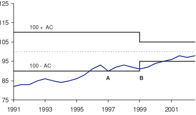
The Constraint for Price Convergence by Arbitrage Cost (AC). The model faces one other difficulty in measuring the euro effect. Arbitrage only functions as a price-convergence device when prices lie outside the band of AC. Figure 3 illustrates the movement of a hypothetical national CPL for an EMU member. The ACs are shown as a lower and upper band around the EMU average to which
the CPL converges over time.19 Once the CPL is within the band of
AC, arbitrage is no longer profitable. At point A the CPL touches the AC band, but in an efficient market arbitrageurs step in and reverse the movement. Membership of EMU can be expected to reduce the AC range for intra-EMU trade (point B), and this triggers further convergence until the CPL is within the band again.
19The simplifying assumption in this example is that the EMU average is equal
The analysis of the euro effect on price convergence relies on the fact that the CPL indices are predominately outside the narrow band at the introduction of the euro as shown in Figure 3. Price convergence might not be observed if CPL indices are already within the narrower (post-EMU) range of AC. The model should ideally test for convergence conditioned on the position of relative prices to the band of ACs. However, the size of the band is unknown in reality.
4. Estimation
4.1 General Results
Of the 161 product groups for which data is of sufficiently high qual-ity, we focused attention on the 115 in the tradable category. As discussed in section 1, price convergence ought to be most appar-ent among tradable goods. Our analysis of the forty-six nontrad-able product groups showed no evidence for a significant decline in price dispersion among EMU countries relative to non-EMU coun-tries. This remained the case when the analysis was restricted to the twenty-nine product groups characterized by relatively low sunk costs.
Following the approach laid out in section 3.3, we begin quantifi-cation of a potential euro effect by estimating equation (2) across the 115 tradable product groups. The results are presented in column 1 in table 5 in the appendix. The model is estimated with product fixed effects and employs the robust variance estimator. The relevant
parameters are the shift coefficient (EM U ·post99) and the trend
coefficient (τ·EM U·post99). The former is insignificant, though
neg-ative, but the latter is significantly negative at the 1 percent level. As expected, we find no instantaneous downward shift in price dis-persion in the euro zone relative to the non-EMU group, consequent to the introduction of the euro. But there is evidence of a downward break in the time trend of price dispersion among EMU countries relative to non-EMU countries after 1999, supporting the hypothesis of a euro effect.
Figure 4. Price Dispersion Difference in (Average Annual) Difference between the Pre-euro Period and the
Euro Period (EMU and Non-EMU)
-0.25 -0.15 -0.05 0.05 0.15 0.25
Edible ice, ice Tea and other O
ther edible
D
elicatessen Fuels and
Pharmaceutical
Fortified and
Miscellaneous Major durables Dried fruit and
Frozen fruit, Por k Other personal Other Other medical Frozen fish Cocoa, Bedroom
Motor cars Ga
rd en s, Clothing Women's Dr ie d
Major tools Motor cars Liquid fuels Unrecorded Hand tools, Other major
Telephone and
Motor cars
Travel goods Non-electric
Pasta products Washing-Infant's O ther meats Small electric Liquefied Product groups CoV (CP
L) : Aver
age annual change in pre-eur
o
per
iod - Aver
age annual ch an g e in eu ro -p erio d
EMU: (avg annual change in Cov in the pre euro period - avg annual change in Cov in the euro period)
Non-EMU: (avg annual change in Cov in the pre euro period - avg annual change in Cov in the euro period )
Difference between EMU and Non-EMU (EMU-Non-EMU) in the difference between pre-euro period average and euro-period average in the annual change in COV
Source: Own calculations using Eurostat data.
These results are mirrored to a large extent in summary compar-isons. In 65 percent of our list of tradable product groups, the euro zone has seen a greater reduction in price dispersion after 1999 than
the non-EMU region.20 In Figure 4 we follow the example of Engel
and Rogers (2004) and present some summary graphical evidence in support of our regression results. We are interested in capturing, in a summary way, the evidence of a trend change (rather than a one-time level change) in price dispersion. We consider year-to-year changes in the coefficient of variation across the country groups, and average these changes for the pre-euro period and for the euro period.
20To illustrate with one example, for the product group comprising washing
We then take away the euro period average annual change from the pre-euro period average annual change, and graph these difference-in-differences to compare the change in price dispersion in the euro zone with that in the non-EMU region (in figure 4 the product groups are arranged in the ascending order of the gap between the euro zone and the non-EMU region). Note that the difference (pre-euro period – euro period) is generally more positive for the euro zone than for the non-EMU region, illustrating unconditional trend re-duction in price dispersion following the launch of the euro.
Over the euro period, the coefficient of variation of CPL, averaged over tradable product groups, fell by 0.5 percent in the euro zone, and rose by 1.2 percent in the non-EMU region. These values are not far from our predictions conditional on the controls in the model—a fall of 0.4 percent in the euro period in the euro zone and a rise of 1 percent in the non-EMU region. However, the trends carry the message—if the trends persist, the difference between the euro zone and the non-EMU region in price dispersion will grow to be starkly evident in just a few years.
4.2 Extracting the Importance of Exchange Rate Risk
EMU incorporates certain exchange rate bands from the preceding Exchange Rate Mechanism (ERM), and not all EMU countries were similar in terms of intragroup trading risk attributable to exchange rate variations in the run up to the euro. The ERM was hit by sev-eral speculative attacks in the aftermath of German reunification in 1990 that led to subsequent interest-rate hikes by the Bundesbank in response to the fiscal expansion. “Black Wednesday” (September 16, 1992) marked the expulsion of Britain and Italy from the ERM.
Fur-ther crises in 1993 led to the adoption of wider (±15 percent) bands
for acceptable fluctuations. Only Germany and Netherlands agreed
bilaterally to remain in the original narrower band of ±2.25
per-cent. Therefore, it could be argued that the exchange rate risk was substantially lower for the German/Netherlands subgroup (G+NL) compared with other EMU members before the introduction of the euro.
Netherlands, and Germany. The exchange rate risk was lower for these DM-zone countries compared with other EMU members before the introduction of the euro.
Separate comparisons of the G+NL and the DM zone against the non-EMU control group should be useful in revealing patterns in convergence. If exchange rate risk increases arbitrage costs sig-nificantly, the DM zone trend coefficient should be smaller (more negative) than the coefficient for the remaining six EMU members. We should expect the G+NL trend coefficient to be negative and closer to zero compared to the coefficient for the remaining nine EMU members, and further, closer to zero than the coefficient for the DM zone. Indeed this is the pattern found in a comparison of the trend coefficients in regressions (3) to (6). The null that the
co-efficient ofτ ·EM U·post99 is equal for EMU and for the DM zone
is rejected decisively:F(1,114) = 42.72,p-value close to 0. However,
though the estimate of the coefficient for the DM zone (−0.036) is
lower than the corresponding estimate for the German/Netherlands
group (−0.031), the null that they are equal for the groups cannot
be rejected:F(1,114) = 1.77, p-value of 0.19.
Overall, these results support the hypothesis that exchange rate risk is a dominant factor in arbitrage costs.
4.3 Nonlinearity in Dispersion Dynamics
We now relax the assumption of linearity in the effect of arbitrage on price dispersion. There are two possible ways in which there may be departures from linearity. One working hypothesis is that the forces of arbitrage will be stronger on (tradable) products that have higher degrees of dispersion. A counterhypothesis to this is that tradable goods may be characterized by differing degrees of “tradability” and price dispersion may be persistently high in those product groups that are inherently “less tradable.”
As a first step in resolving this issue, we estimate equation (3) across all tradables. Table 6 in the appendix presents the results. The coefficients of interest are those on the lagged dispersion quartile
dummy variablesQ1, Q2, Q3,andQ4 interacted with the time-trend
the higher quartiles. The results are the opposite. For EMU, and subgroups of EMU, the interacted coefficients on the higher quar-tiles are very significantly (almost always at 1 percent) larger (closer
to zero) than those on the lower quartiles.21 The differentiated
pat-terns in high and low price dispersion product groups seem to be such that high-dispersion product groups consistently converge less than low-dispersion product groups.
To explore this further, we examine a select set of broad product categories to distinguish between the less and more tradable product groups. For example, food can be separated out into perishable food products (e.g., bread, fresh fish, fresh fruit) that are less tradable, and nonperishable food products (e.g., sugar, coffee). It might be ex-pected that the pressure on prices to converge will be lower for per-ishable food products than for nonperper-ishable food products. Again, electrical appliances (e.g., washing machines, ovens, hand tools) are highly tradable. Alcohol and tobacco products, while highly trad-able in principle, are marked by country-specific excise taxes. There is less reason to expect that reduced arbitrage costs will reduce price differences between countries for the latter. Table 7 in the appendix presents the results for the product groups (table 3) in these broad categories.
The smaller number of observations at product category level re-duces the resolution with which patterns emerge. In column 1 the results for perishable food show that the trend coefficient is not sig-nificantly different from zero. In contrast, for nonperishable food, a significant (at 10 percent) tendency towards reduced dispersion can be observed (column 2). Alcohol and tobacco have no signifi-cant tendency toward reduced price dispersion, while electrical ap-pliances show a strong convergent tendency (significant at 5 percent; column 4).
5. Conclusion
Our objective was to test the hypothesis that the euro has had a positive effect on price convergence among EMU members relative
21It was in the case of the DM zone that the pattern was least strong: the
to non-EMU members. Our findings suggest that this is true. The process of convergence in the euro zone triggered by EMU appears in the form of a structural break in the time trend of price disper-sion. For EMU, this break accelerates the evident general trend of reduction in price dispersion across all EU countries after 1995.
Policymakers anticipated declines in price dispersion following the launch of the euro, but the first tranche of academic research papers on this topic did not find evidence of price convergence after 1999, over and above the convergence patterns evident from the early 1990s. Our finding stands in sharp contrast to this literature, and would indicate that the euro zone has moved further along in achiev-ing a sachiev-ingle market, relative to EU countries outside the euro zone. A clearer understanding of the welfare effects of EMU should follow from examining whether product prices converge to their respective lowest price in the EMU.
Variations in the ERM history of the EU members permit us to examine the importance of exchange rate risk for arbitrage costs. We find that the magnitude of the euro effect depends on the extent of pre-EMU exchange rate risk. It may be interesting to explore whether different expectations of EU members joining the euro in the run up to the EMU were relevant to the euro effect.
In te rn at ion al J ou rn al of C en tr al B an k in g D ec em b er 2005 e n d ix
Table 1. A Survey of Empirical Evidence on Purchasing Power Parity and the Law of One Price
Author(s) and Date Time Period Data Source Countries/Cities Product(s) Results:Mixed
Beck & Weber (2003)
1991–2002 SPAT-DAT regional
81 European cities in 7 countries
Price index and 10 categories of consumer goods
Border effects greater than distance. Unit root test shows faster convergence. After EMU, intranational price dispersion falls 80%.
Imbs et al. (2004) 1999–2002 GfK (French Survey Company)
15 EU plus Poland, Hungary, and Czech Republic
3 categories of TV sets
Price dispersion lower in EMU but most of this achieved before 1999. Regions more integrated than countries.
Lutz (2004) 1993–1998 EU Commission 12 countries 90 cars Price differentials affected by language, common border, and low trade barriers. Belgian/ Luxembourg currency union 4% lower price differential.
Lutz (2003) 1987–2001 1995–2001 1995–2001 1970–2000 The Economist, The Economist, EU Commission, UBS 11 countries 20 countries 12 countries 19 cities
1 Big MacR
1The Economist
17 cars 13 categories
OnlyThe Economistmagazine showed price convergence. Euro did not speed convergence either.
Math¨a (2003) 2001–2002 (four points)
Authors’ own City of Luxembourg and contiguous regions in four countries
92 products from 6 supermarkets
Monetary union shows price convergence. If distance rises 1% then prices rise 0.025%. Distances smaller in EMU than US, so room for optimism.
Parsley & Wei (2001) 1990–2000 Economist Intelligence Unit (EIU)
1 N o. 3 O n e M ar k et , O n e M on ey , O n e P ric e? 99
Table 1 (continued). A Survey of Empirical Evidence on Purchasing Power Parity and the Law of One Price
Author(s) and Date Time Period Data Source Countries/Cities Product(s) Results:Negative
Baye et al. (forthcoming)
October 2001– May 2002
Kelkoo Internet prices
7 countries of which 4 in euro zone
28 products Price dispersion in EU slightly lower than for comparable goods in U.S. End-of-period euro zone prices 10% higher than non-euro zone.
Engel & Rogers (2004)
1990–2002/3 EIU 18 cities (11 EMU, 7 outside)
139 Non-euro zone mimics euro zone and increase in dispersion larger. Price dispersion falls during 1990s but little after 1999. After 1998, dispersion for tradables increases.
Goldberg & Verboven (2004)
1970–2000 Authors’ own Belgium, France, Germany, Italy, and United Kingdom
150 vehicle makes
Convergence of prices 1990–92 but divergence thereafter, particularly UK and Italy. Half life of 1.3 years (absolute version 8.3 years).
Rogers (2002) 1990–2001 EIU 25 EU and 13 U.S. cities
139 goods Fall in EU price dispersion mostly before 1994; EU level close to that in US 2001. EMU cities same result.
Results:Positive
Isgut (2002) 2001 EIU 122 cities in OECD 140 goods and
services
Same currency reduces log of price differences across cities 2–3%, for EU group 5%. Dollar peg or hard peg same effect.
Friberg & Math¨a (2004)
October 2001– April 2003
Authors’ own Contiguous regions to Luxembourg in 4 countries
92 supermarket products
[image:28.612.157.654.164.432.2]In
te
rn
at
ion
al
J
ou
rn
al
of
C
en
tr
al
B
an
k
in
g
D
ec
em
b
er
[image:29.612.161.637.151.433.2]2005
Table 2. Product Groups Divided into Tradables (T) and Nontradables (NT)
Product Group: Basic Heading Category Product Group: Basic Heading Category
Rice T Cookers, hobs, and ovens T
Flour and other cereals T Air conditioners, humidifiers, and heaters T
Bread T Other major household appliances T
Other bakery products T Small electric household appliances T
Pasta products T Repair of household appliances NT
Other cereal products T Glassware and ceramic ware for households,
offices, and decoration
T
Beef T Cutlery, flatware, and silverware T
Veal T Nonelectric kitchen utensils and household
articles
T
Pork T Major tools and equipment T
Lamb, mutton, and goat T Small electric accessories T
Poultry T Hand tools, garden tools, and other
miscellaneous accessories
T
Other meats and edible offal T Household cleaning supplies T
Delicatessen and other meat preparations T Other non-durable household articles T
Fresh or chilled fish and seafood T Domestic services NT
1
N
o.
3
O
n
e
M
ar
k
et
,
O
n
e
M
on
ey
,
O
n
e
P
ric
e?
101
Nontradables (NT)
Product Group: Basic Heading Category Product Group: Basic Heading Category
Preserved or processed fish and seafood T Other household services NT
Fresh milk T Pharmaceutical products T
Preserved milk T Other medical products T
Other milk products T Eyeglasses and contact lenses T
Cheese T Other therapeutic appliances and equipment T
Eggs and egg-based products T H — Compensation of employees: physicians NT
Butter T H — Compensation of employees: nurses and
other medical staff
NT
Margarine T H — Compensation of employees: nonmedical
staff
NT
Other edible oils and fats T Motor cars with diesel engine T
Fresh or chilled fruit T Motor cars with petrol engine of cubic
capacity of less than 1200cc
T
Dried fruit and nuts T Motor cars with petrol engine of cubic
capacity of 1200cc to 1699cc
T
Frozen fruit, preserved fruit, and fruit-based products
T Motor cars with petrol engine of cubic
capacity of 1700cc to 2999cc
T
Fresh or chilled vegetables other than potatoes
T Motor cars with petrol engine of cubic
capacity of 3000cc and over
[image:30.612.162.634.161.440.2]In
te
rn
at
ion
al
J
ou
rn
al
of
C
en
tr
al
B
an
k
in
g
D
ec
em
b
er
2005
Nontradables (NT)
Product Group: Basic Heading Category Product Group: Basic Heading Category
Fresh or chilled potatoes T Motorcycles T
Frozen vegetables T Bicycles T
Dried vegetables T Spare parts and accessories for personal
transport equipment
T
Preserved or processed vegetables and vegetable-based products
T Fuels and lubricants for personal transport
equipment
T
Sugar T Maintenance and repair of personal
transport equipment
NT
Jams, marmalades, and honey T Other services in respect of personal
transport equipment
NT
Confectionery, chocolate, and other cocoa preparations
T Local passenger transport by railway NT
Edible ice, ice cream, and sorbet T Long-distance passenger transport by railway NT
Food products n.e.c. T Local passenger transport by bus NT
Coffee T Local passenger transport by taxi NT
Tea and other infusions T Long-distance passenger transport by road NT
Cocoa, excluding cocoa preparations T Passenger transport by air NT
Mineral waters T Passenger transport by sea and inland
waterway
[image:31.612.164.636.160.441.2]1
N
o.
3
O
n
e
M
ar
k
et
,
O
n
e
M
on
ey
,
O
n
e
P
ric
e?
103
Nontradables (NT)
Product Group: Basic Heading Category Product Group: Basic Heading Category
Soft drinks and concentrates T Other purchased transport services NT
Fruit and vegetable juices T Postal services NT
Spirits T Telephone and telefax equipment T
Wine, cider, and perry T Telephone and telefax services NT
Fortified and sparkling wine T Television sets and video recorders T
Beer T Radios, CD players, and other
electro-acoustic devices
T
Cigarettes T Photographic and cinematographic
equipment and optical instruments
T
Other tobacco products T Information processing equipment T
Clothing materials T Prerecorded recording media T
Men’s clothing T Unrecorded recording media T
Women’s clothing T Repair of audio-visual, photographic, and
information processing equipment
NT
Children’s clothing T Major durables for outdoor recreation T
Infant’s clothing T Musical instruments and major durables for
indoor recreation
T
Other articles of clothing and clothing accessories
T Maintenance and repair of other major
durables for recreation and culture
[image:32.612.162.639.158.443.2]In
te
rn
at
ion
al
J
ou
rn
al
of
C
en
tr
al
B
an
k
in
g
D
ec
em
b
er
2005
Nontradables (NT)
Product Group: Basic Heading Category Product Group: Basic Heading Category
Cleaning, repair, and hire of clothing NT Games, toys and hobbies T
Men’s footwear T Equipment for sport, camping, and open-air
recreation
T
Women’s footwear T Gardens, plants, and flowers T
Children’s and infant’s footwear T Pets and related products T
Repair and hire of footwear NT Veterinary and other services for pets NT
Actual rentals paid by tenants living in apartments
NT Recreational and sporting services NT
Actual rentals paid by tenants living in one-family houses
NT Photographic services NT
Imputed rentals of owner-occupiers living in apartments
NT Other cultural services NT
Imputed rentals of owner-occupiers living in one-family houses
NT Books NT
Materials for the maintenance and repair of the dwelling
T Newspapers and periodicals NT
Services for the maintenance and repair of the dwelling
NT Miscellaneous printed matter T
Water supply NT Stationery and drawing materials T
Electricity NT Restaurant services whatever the type of
establishment
[image:33.612.162.641.151.448.2]1
N
o.
3
O
n
e
M
ar
k
et
,
O
n
e
M
on
ey
,
O
n
e
P
ric
e?
105
Nontradables (NT)
Product Group: Basic Heading Category Product Group: Basic Heading Category
Town gas and natural gas NT Pubs, bars, caf´es, tea rooms and the like NT
Liquefied hydrocarbons T Other catering services NT
Liquid fuels T Canteens NT
Solid fuels T Hotels, boarding houses, and the like NT
Kitchen furniture T Other accommodation services NT
Bedroom furniture T Services of hairdressers and the like for men NT
Living-room and dining-room furniture T Services of hairdressers and the like for
women
NT
Other furniture and furnishings T Electric appliances for personal care T
Carpets and other floor coverings T Other appliances, articles, and products for
personal care
T
Repair of furniture, furnishings, and floor coverings
NT Jewelery, clocks, and watches T
Household textiles T Travel goods and other carriers of personal
effects
T
Refrigerators, freezers, and fridge-freezers T Other personal effects n.e.c. T
Washing machines, dryers, and dishwashers T
[image:34.612.161.636.161.434.2]Table 3. Selected Product Groups
Food: Perishable
Bread Fresh milk
Other bakery products Preserved milk
Pasta products Other milk products
Other cereal products Cheese
Beef Eggs and egg-based products
Veal Butter
Pork Margarine
Lamb, mutton, and goat Other edible oils and fats
Poultry Fresh or chilled fruit
Other meats and edible offal Fresh or chilled vegetables other
than potatoes
Delicatessen and other meat preparations
Fresh or chilled potatoes
Fresh or chilled fish and seafood Frozen vegetables
Frozen fish and seafood Preserved or processed vegetables
and vegetable-based products
Preserved or processed fish and seafood
Edible ice, ice cream, and sorbet
Food: Nonperishable
Flour and other cereals Coffee
Dried fruit and nuts Tea and other infusions
Frozen fruit, preserved fruit, and fruit-based products
Cocoa, excluding cocoa preparations
Dried vegetables Mineral waters
Sugar Soft drinks and concentrates
Jams, marmalades, and honey Fruit and vegetable juices
Table 3 (continued). Selected Product Groups
Alcohol and Tobacco
Spirits Beer
Wine, cider, and perry Cigarettes
Fortified and sparkling wine Other tobacco products
Electrical Appliances
Refrigerators, freezers, and fridge-freezers
Small electric accessories
Washing machines, dryers, and dishwashers
Telephone and telefax equipment
Cookers, hobs, and ovens Television sets and video recorders
Air conditioners, humidifiers, and heaters
Radios, CD players, and other electro-acoustic devices
Other major household appliances Photographic and
cinemato-graphic equipment and optical instruments
Small electric household appliances Information processing equipment
Major tools and equipment Electric appliances for personal
[image:36.612.126.449.161.433.2]Table 4. The National Comparative Price Level (CPL) Indices Relative to the EU Mean of 100
National CPL
(EU15=100) 1995 1996 1997 1998 1999 2000 2001 2002
Austria 111.8 107.7 103.4 103.4 101.7 99.5 101.2 101.6
Belgium 108.7 105.3 102.3 102.3 102.6 100.3 98.9 98.2
Denmark 132.1 129.8 126.8 126.1 123.5 122.8 123.3 126.1
Finland 115.0 110.6 107.6 106.9 107.3 106.6 107.4 109.8
France 108.7 107.2 102.5 102.1 101.3 99.6 99.0 98.7
Germany 120.8 115.6 111.1 110.6 109.6 106.8 107.4 106.8
Greece 73.4 76.2 78.0 75.9 77.8 75.4 76.4 75.7
Ireland 89.0 91.6 97.0 96.9 100.6 103.8 108.4 109.7
Italy 79.5 87.8 89.8 88.4 88.4 88.0 90.1 91.8
Luxembourg 118.3 115.4 112.3 111.2 107.3 107.6 109.8 110.5
Netherlands 106.9 103.5 99.7 100.1 101.1 100.7 101.1 102.7
Portugal 70.6 71.6 71.2 71.2 70.9 70.8 72.4 73.3
Spain 81.5 83.1 81.2 80.9 80.1 80.8 82.5 82.9
Sweden 113.8 122.2 120.1 117.6 115.8 118.5 111.0 113.9
United Kingdom 84.8 86.2 99.9 103.7 106.8 113.0 110.4 108.4
Table 5. Regression Results
DM Zone: EMU Less EMU Less Treatment Group EMU (A+B+G+L+N) DM Zone G+N G+N Control Group Non-EMU Non-EMU Non-EMU Non-EMU Non-EMU
Equation 1 2 3 4 5 6
EMU† −0.101 −0.101 −0.139 −0.106 −0.154 −0.103
(3.60)∗∗ (4.92)∗∗ (10.19)∗∗ (3.62)∗∗ (8.98)∗∗ (4.62)∗∗ post1999 −0.004 −0.004 0.006 −0.012 0.002 −0.005 (0.27) (0.38) (0.55) (1.28) (0.20) (0.49)
EMU*post1999 −0.005 −0.005 −0.002 −0.006 −0.011 −0.003 (0.32) (0.41) (0.14) (0.41) (0.75) (0.23)
τ −0.035 −0.035 −0.034 −0.039 −0.03 −0.036
(6.04)∗∗ (7.81)∗∗ (8.08)∗∗ (8.10)∗∗ (8.80)∗∗ (8.05)∗∗
τ *EMU 0.03 0.03 0.029 0.033 0.029 0.031
(3.38)∗∗ (5.15)∗∗ (7.90)∗∗ (4.59)∗∗ (6.46)∗∗ (5.09)∗∗
τ *post1999 0.05 0.05 0.043 0.06 0.036 0.052 (4.07)∗∗ (6.08)∗∗ (6.34)∗∗ (6.40)∗∗ (5.70)∗∗ (6.33)∗∗
τ *EMU*post1999 −0.04 −0.04 −0.036 −0.048 −0.031 −0.042 (2.80)∗∗ (4.30)∗∗ (5.43)∗∗ (4.31)∗∗ (3.91)∗∗ (4.47)∗∗ Std Dev Real GDP 1.316 1.316 0.29 2.325 0.361 1.466
Growth Rate
(2.01)∗ (3.85)∗∗ (2.02)∗ (3.91)∗∗ (1.20) (4.04)∗∗ Std Dev CP Index 1.629 1.629 1.171 2.557 0.13 1.812
Growth Rate
(1.28) (1.94) (1.53) (2.85)∗∗ (0.28) (2.20)∗
Std Dev Real −0.009 −0.009 −0.007 −0.012 −0.004 −0.009
Exchange Rate
(0.39) (0.86) (0.70) (1.18) (0.38) (0.93)
Constant 0.271 0.271 0.284 0.264 0.299 0.271 (8.68)∗∗ (22.99)∗∗ (25.01)∗∗ (21.71)∗∗ (27.31)∗∗ (22.91)∗∗ Product Fixed Yes Yes Yes Yes Yes Yes
Effects
R-squared 0.52 0.52 0.5 0.52 0.5 0.52
Observations 1840 1840 1840 1840 1840 1840
Estimation Robust Robust, premitting clustering by product groups
Notes:Robust t statistics in parentheses;∗significant at 5%;∗∗significant at 1%. †The EMU dummy denotes dummy of the treatment group; i.e. the DM zone comprising
Table 6. Regression Results: Nonlinearity in Covergence
DM Zone: EMU Less EMU Less Treatment Group EMU (G+A+B+N+L) DM Zone G+N G+N Control Group Non-EMU Non-EMU Non-EMU Non-EMU Non-EMU
Equation 1 2 3 4 5
EMU† −0.109 −0.144 −0.107 −0.176 −0.114
(3.87)∗∗ (9.65)∗∗ (3.68)∗∗ (8.23)∗∗ (5.24)∗∗
post1999 −0.002 0.008 −0.011 0.001 −0.002
(0.14) (0.70) (1.19) (0.11) (0.22)
EMU*post1999 −0.007 −0.003 −0.005 −0.014 −0.005
(0.40) (0.24) (0.38) (0.97) (0.40)
τ −0.037 −0.036 −0.038 −0.033 −0.039
(6.17)∗∗ (7.90)∗∗ (7.30)∗∗ (8.22)∗∗ (8.57)∗∗
τ *EMU 0.033 0.031 0.034 0.035 0.034
(3.61)∗∗ (7.54)∗∗ (4.54)∗∗ (6.40)∗∗ (5.71)∗∗
τ *post1999 0.052 0.046 0.058 0.04 0.055 (4.18)∗∗ (6.53)∗∗ (5.96)∗∗ (5.96)∗∗ (6.77)∗∗
τ *EMU*post1999*Q1 −0.056 −0.049 −0.067 −0.05 −0.061 (3.89)∗∗ (7.03)∗∗ (6.04)∗∗ (5.88)∗∗ (6.73)∗∗
τ *EMU*post1999*Q2 −0.05 −0.045 −0.053 −0.044 −0.053 (3.49)∗∗ (6.70)∗∗ (4.84)∗∗ (5.11)∗∗ (5.73)∗∗
τ *EMU*post1999*Q3 −0.04 −0.039 −0.046 −0.035 −0.044 (2.76)∗∗ (5.61)∗∗ (4.35)∗∗ (4.07)∗∗ (4.82)∗∗
τ *EMU*post1999*Q4 −0.024 −0.02 −0.024 −0.015 −0.024 (1.65) (2.83)∗∗ (1.85) (1.50) (2.42)* Std Dev Real GDP 1.247 0.26 2.204 0.585 1.4
Growth Rate
(1.99)∗ (1.92) (3.69)∗∗ (1.45) (4.08)∗∗
Std Dev CP Index 1.547 1.241 2.267 0.005 1.788
Growth Rate
(1.22) (1.66) (2.41)∗ (0.01) (2.18)∗ Std Dev Real Exchange −0.009 −0.008 −0.011 −0.005 −0.01
Rate
(0.41) (0.79) (1.10) (0.46) (1.02)
Constant 0.284 0.296 0.271 0.303 0.287 (9.19)∗∗ (22.97)∗∗ (19.61)∗∗ (22.50)∗∗ (21.73)∗∗ Product Fixed Effects Yes Yes Yes Yes Yes
R-squared 0.55 0.52 0.56 0.52 0.56
Observations 1786 1791 1767 1738 1795
Notes:Robust t statistics in parentheses;∗significant at 5%;∗∗significant at 1%.
†See table 1 for intrepretation of the EMU dummy.
Table 7. Regression Results: Selected Product Groups
Perishable Nonperishable Alcohol and Electrical Food food Tobacco Appliances
Equation 1 3 5 7
EMU −0.053 −0.158 0.106 −0.218
(1.51) (2.28)* (2.28)+ (5.40)**
post1999 −0.013 0.006 0.007 0.012
(0.83) (0.20) (0.21) (0.52)
EMU*post1999 0 −0.038 −0.074 0.01
(0.01) (0.77) (1.56) (0.41)
τ −0.02 −0.038 −0.011 −0.064
(3.26)** (3.52)** (0.87) (5.33)**
τ *EMU 0.012 0.043 0.01 0.056
(1.28) (2.55)* (0.79) (3.59)**
τ *post1999 0.014 0.037 0.022 0.085
(1.18) (3.32)** (1.43) (2.52)*
τ *EMU*post1999 0.001 −0.031 0.004 −0.081
(0.08) (1.91)+ (0.18) (2.19)*
Std Dev Real GDP 0.442 1.963 2.096 2.934
Growth Rate
(0.76) (1.85)+ (1.16) (4.01)**
Std Dev CP Index −1.207 2.034 1.644 3.719
Growth Rate
(0.72) (0.62) (0.45) (1.56)
Std Dev Real 0.006 0.018 −0.019 0.035
Exchange Rate
(0.60) (1.13) (0.78) (0.81)
Constant 0.289 0.21 0.268 0.322 (11.71)** (6.46)** (3.69)* (19.34)**
Product Fixed Effects Yes Yes Yes Yes
R-squared 0.4 0.53 0.67 0.48
Observations 448 224 96 224
Notes:Robust t statistics in parentheses; + significant at 10%; * significant at 5%; ** significant at 1%.
In all equations, the treatment group is EMU and the control group comprises the non-EMU countries.
References
Balassa, Bela. 1964. “The Purchasing Power Parity Doctrine: A
Re-Appraisal.”Journal of Political Economy 72:584–96.
Baye, Michael, Rupert Gatti, Paul Kattuman, and John Morgan. Forthcoming. “Online pricing and the euro changeover:
Cross-country comparisons.” Forthcoming in Economic Inquiry.
Beck, Guenter, and Axel A. Weber. 2003. “How Wide Are European Borders? On the Integration Effects of Monetary Unions.” Work-ing Paper No. 2001/07, Centre for Financial Studies, Frankfort, Germany. A revised version of a paper published first in 2001. Begg, David, Jurgen von Hagan, Charles Wyplosz, and Klaus
Zimmerman. 2001.EMU: Prospects and Challenges for the Euro.
London: Centre for Policy Research.
Bertrand, Marianne, Esther Duflo, and Sendhil Mullainathan. 2004. “How Much Should We Trust Differences-in-Differences
Estimates? Quarterly Journal of Economics 119 (1): 249–75.
Cecchetti, Stephen, Nelson C. Mark, and Robert Sonora. 1999. “Price Level Convergence Among United States Cities: Lessons for the European Central Bank.” NBER Working Paper No. 7681.
Eleftheriou, Maria. 2003. “On the Robustness of the ‘Taylor Rule’ in the EMU.” Working Paper No. ECO2003/17, Department of Economics, European University Institute, San Domenico di Fiesole, Italy.
Engel, Charles, and John H. Rogers. 1996. “How Wide is the
Border?” American Economic Review 86:1112–25.
———. 2004. “European Product Market Integration After the
Euro.”Economic Policy (July):347–84.
European Commission. 1990. “One market, one money: An evalua-tion of the potential benefits and costs of forming an economic
and monetary union.” European Economy 44 (October).
———. 1996. “The 1996 single market review — background infor-mation for the report to the Council and European Parliament.” Commission Staff Working Paper, SEC (96) 2378, (December 16), Brussels, Belgium.