Analysis the Results of Acoustic Echo
Cancellation for Speech Processing using LMS
Adaptive Filtering Algorithm
Ranbeer Tyagi
Department of Electronics & Comm. Engg. PCRT (PU), Bhopal (M.P.) India
Dheeraj Agrawal
Department of Electronics & Comm. Engg. MANIT, Bhopal (M.P.) India
ABSTRACT
The Conventional acoustic echo canceller encounters problems like slow convergence rate (especially for speech signal) and high computational complexity as the identification of the echo path requires filter with more than a thousand taps, non-stationary speech input, slowly time-varying systems to be identified. The demand for fast convergence and less MSE level cannot be met by conventional adaptive filtering algorithms. There is a need to be computationally efficient and rapidly converging algorithm.
The LMS algorithm is easy to implement and computationally inexpensive. This feature makes the LMS algorithm attractive for echo cancellation applications. The results show that the steady state value of the output estimation error increases with increasing the step size parameter and the optimality of the LMS algorithm is no longer hold. The results also reveal that choosing the smallest value of the step size parameter guarantees the smallest mis-adjustment but might not meet the convergence criteria.
General Terms
Adaptive Filtering Algorithm, Acoustic Echo-cancellation.
Keywords
LMS Algorithm, Echo-cancellation, ERLE, MSE.
1.
INTRODUCTION
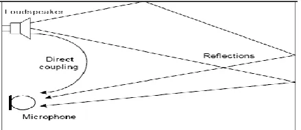
Teleconferencing systems are expected to provide a high sound quality. Speech by the far end speaker is captured by the near end microphone and being sent back to him as echo. Acoustic echoes cause great discomfort to the users since their own speech (delayed version) is heard during conversation. The echo has been a big issue in communication networks. Hence this is devoted to the investigation and development of an effective way to control the acoustic echo in hands-free communications [1]. The Generation of acoustic echo through direct coupling and reverberations [2] can be shown in Fig. 1. Each side of the communication process is called an ‘End’. The remote end from the speaker is called the far end (FE), and the near end (NE) refers to the end being measured. The acoustic echo is due to the coupling between the loudspeaker and microphone.
The speech of the far-end speaker is sent to the loudspeaker at the near end, and it is reflected from the floor, walls and other neighboring objects, and then picked up by the near-end microphone and transmitted back to the far-end speaker, yielding an echo, which can be illustrated in Figure 1.
The paper is organized as follows. Section 2 presents the principles of acoustic echo cancellation in teleconferencing
[image:1.595.320.540.297.392.2]environment. Section 3, 4 gives a very brief idea about Discrete Time Signal and Speech Signal. Section 5, 6 gives a very brief review on The LMS Algorithm. Section 7 reports the Discussion and Analysis of Simulation results, carried out on acoustic echo cancellation using LMS Algorithm. The conclusions and references are discussed in the last Section.
Fig 1: Generation of acoustic echo through direct coupling and reverberations
2.
THE PRINCIPLES OF ACOUSTIC
ECHO CANCELLATION
In a teleconferencing environment, speech by the near end speaker is often captured by the far end microphone and being sent back to him as echo. For acoustic echo cancellation, the initial speech transmitted to the far end is adaptively filtered to follow the echo of the speech retransmitted from the far end. The difference of the two signals (i.e. the error of the adaptive filter) is transmitted to the near end [20]. This error signal is used by the adaptive filter in adapting its filter parameters. Figure 2 shows such an acoustic echo cancelling setup. Referring to figure let x(n) be the input signal (from the far end speaker) travelling to the near end speaker through the loudspeaker and d(n) is the signal picked up by the microphone which in this case is the far end echo corrupted with noise .
The adaptive filter is used to model the transfer function of the room in which the loudspeaker and microphone are in to generate a replica of the echo, y(n) following that, the estimated echo is subtracted from the desired input signal d(n) yielding the estimation error signal,
e
(
n
)
d
(
n
)
y
(
n
)
1Simply, the adaptive filter is self adjusting hence the name ‘adaptive’.
[image:2.595.60.274.151.272.2]In an acoustic echo cancellation [3], [14], [18], a model of the room impulse response may vary continuously hence the model needs to be updated continuously. This is done by means of adaptive filtering algorithms.
Fig 2: Acoustic Echo Canceller configurations
3.
DISCRETE TIME SIGNAL
Real world signals, such as speech are analog and continuous. An audio signal, as heard by our ears is a continuous waveform which derives from air pressure variations fluctuating at frequencies which we interpret as sound. However, in modern day communication systems these signals are represented electronically by discrete numeric sequences [4]. In these sequences, each value represents an instantaneous value of the continuous signal. These values are taken at regular time periods [5], known as the sampling period, Ts.
The values of the sequence, x(t) corresponding to the value at n times the sampling period is denoted as x(n).
)
(
)
(
n
x
nT
sx
24.
SPEECH SIGNAL
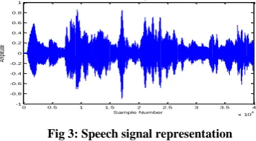
[image:2.595.327.541.171.306.2]A speech signal consists of three classes of sounds [13]. They are voiced, fricative and plosive sounds. Voiced sounds are caused by excitation of the vocal tract with quasi-periodic pulses of airflow. Fricative sounds are formed by constricting the vocal tract and passing air through it, causing turbulence that result in a noise-like sound. Plosive sounds are created by closing up the vocal tract, building up air behind it then suddenly releasing it. This is heard in the sound made by the letter. Figure 3 shows a discrete time representation of a speech signal.
Fig 3: Speech signal representation
5.
THE LMS ALGORITHM
The LMS algorithm is a type of adaptive filter known as stochastic gradient-based algorithms as it utilizes the gradient vector of the filter tap weights to converge on the optimal wiener solution. It is well known and widely used due to its computational simplicity [6].
LMS algorithm consists of two basic processes
1. A filtering process- which involves computing the output d(n) of the Transversal filter generating from the set of tap weights, and computing a error e(n) by comparing this output with the actual desired response.
2. An adaptive process- which involves the automatic adjustment of the tap weights. Figure 4 shows the block diagram of adaptive transversal filter.
Fig 4: Block diagram of Adaptive Transversal Filter
The filter tap weights of the adaptive filter LMS algorithm [6], [7] are updated according to this equation
w
(
n
1
)
w
(
n
)
e
(
n
)
x
(
n
)
3Where w (n) is the tap weight vector at time n.
The parameter µ is known as the step size parameter and is a small positive constant. This step size parameter controls the influence of the updating factor. Selection of a suitable value for is imperative to the performance of the LMS algorithm, if the value is too small the time the adaptive filter [8] takes to converge on the optimal solution will be too long; if µ is too large the adaptive filter becomes unstable and its output diverges.
It is noted that the existence of feedback e(n) in the LMS Algorithm [19] may cause the algorithm to be unstable. Fortunately, the stability of the algorithm can be determined by the step-size parameter. The step size parameter should satisfy the following
max
2
0
S
4Where
S
maxis maximum value of input signal power.6.
ANALYSIS OF THE LMS
ALGORITHM
The LMS algorithm minimizes the expected value of the squared error (residual echo). Thus the criterion function, mean squared error is
)]
(
[
e
2n
E
J
5)]
(
[
e
2n
E
J
)]
(
[
)
(
2
e
n
E
e
n
J
)]
(
)
(
)
(
[
)
(
2
e
n
E
d
n
W
n
x
n
J
T
0 0.5 1 1.5 2 2.5 3 3.5 4x 10⁴ -1
-0.8 -0.6 -0.4 -0.2 0 0.2 0.4 0.6 0.8 1
Am
pli
tu
de
Sample Number Far End Speech
Transversal
Filter [w (n)]
Adaptive Weight
Control Mechanism
)
(
n
x
)
(
n
y
[image:2.595.65.251.591.693.2])
(
)
(
2
e
n
x
n
J
6For simplicity, the tap input vector x(n) and the desired response d(n) are assumed to be jointly wide-sense stationary [9]. With this assumption, the method of steepest descent can be used to compute a tap weight vector.
J
n
w
n
w
(
1
)
(
)
7)
(
)
(
2
)
(
)
1
(
n
w
n
e
n
x
n
w
8For convenience, the factor two in equation 8 is absorbed into the constant µ yielding
)
(
)
(
)
(
)
1
(
n
w
n
e
n
x
n
w
9The LMS algorithm has a correction factor of µ e(n)x(n) to the tap weight vector w(n). One notable fact is that the correction factor is directly proportional to the tap input vector x(n) and hence when x(n) is large, the LMS algorithm faces a gradient noise amplification problem [10]. This means the error in the gradient estimate gets magnified.
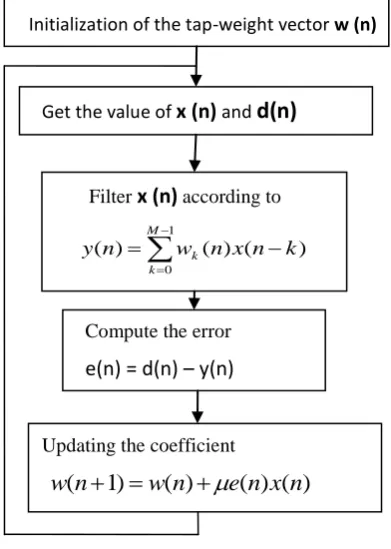
The main reason for the LMS algorithms popularity in adaptive filtering is its computational simplicity, making it easier to implement than all other commonly used adaptive algorithms. For each iteration the LMS algorithm requires 2N additions and 2N+1 multiplications (N for calculating the output, y(n), one for 2μe(n) and an additional N for the scalar by vector multiplication) [11], [12], [17]. Figure 5 shows the flowchart of the basic LMS adaptive filtering Algorithm.
Fig 5: Flowchart of the Basic LMS Algorithm
7.
DISCUSSION AND ANALYSIS OF
SIMULATION RESULTS
The LMS algorithm was simulated using Matlab with respect to the application of acoustic echo cancellation depicted in Figure 2. LMS algorithm is easy to implement and computationally inexpensive. This feature makes the LMS
algorithm attractive for echo cancellation applications. Simulations involving real speech input signal consisted of 48,000 sample points and the echo path was assumed to have known impulse response, h(n) of 500 points long.
Table 1 shows the condition of simulation experiment for LMS Algorithm for acoustic echo cancellation [15, 16].
In this paper filter length was taken to be 300 taps. The parameter of LMS algorithm µ was set to be 0.03 and the near end speaker was assumed to be noisy. Noise variance was set at 0.012.
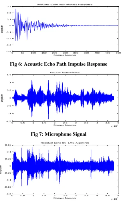
Figure 6 shows the Acoustic echo path Impulse from where Output of Loudspeaker is passed. Figure 7 shows Microphone Signal which is Resulting Far End Echo corrupted with Noise from near end. Residual Echo of LMS filter is shown in Figure 8 and it is compared with Microphone signal in Figure 9. It can be seen that the residual echo is small but not satisfactory. Mean square error performance is shown in Figure 10 which is showing the average of the MSE decay to zero after long time [11].
A very useful tool to express the effect of echo cancellation is the Echo Return Loss Enhancement (ERLE) [12] defined as:
))
(
(
))
(
(
log
10
2 2
n
e
E
n
d
E
ERLS
dB
10 [image:3.595.61.257.397.672.2]Where, E represents the estimated expected value by means of moving averages. Here, the ERLE is used as the performance index of the algorithm and is defined as the ratio of energy in the original echo d (n) to the energy in the residual echo e (n).
Table 1. Condition of Simulation Experiment using fixed values of µ
Simulation Parameters Value
Time (length of signal in second) 6 sec
Sample Rate of speech Signal 8KHz
LMS Step size (µ) 0.03
No of adaptive Filter Tap 300
Moving point average (Mpa) 150
length of room impulse response (M) 500
[image:3.595.315.540.432.536.2]Noise Variable 0.012
Table 2. Condition of Simulation Experiment using different values of µ
Simulation Parameters Value
Time (length of signal in second) 6 sec
Sample Rate of speech Signal 8KHz
LMS Step size (µ) 0.001, 0.007,
0.03
No of adaptive Filter Tap 300
Moving point average (Mpa) 150
length of room impulse response (M) 500
Noise Variable 0.012
In other words, ERLE is a measure of how much echo is attenuated in decibel (dB).
ERLE for LMS algorithm is shown in Figure 11.It is observed that the ERLE for LMS algorithm has lower peaks hence convergence is slower as well as less echo suppression is achieved.
Initialization of the tap-weight vector w (n)
Get the value of
x (n)
andd(n)
Filter x (n)according to
)
(
)
(
)
(
1
0
k
n
x
n
w
n
y
M
k
k
Compute the error
e(n) = d(n) – y(n)
( ) ( ) ( )
Updating the coefficient
)
(
)
(
)
(
)
1
(
n
w
n
e
n
x
n
Fig 6: Acoustic Echo Path Impulse Response
Fig 7: Microphone Signal
Fig 8: Residual Echo of LMS Algorithm
Fig 9: Comparison of Microphone Signal with remaining Residual Echo of LMS Algorithm
[image:4.595.330.534.74.166.2]Fig 10: MSE Performance of LMS Algorithm
Fig 11: ERLE Performance of LMS Algorithm
[image:4.595.325.546.259.451.2]The convergence behaviour of the LMS algorithm is highly dependent on the step size parameter µ. As an illustration, the learning curves of ERLE and MSE for three different values of µ (.001, .007 and .03) are depicted in Figure 12 and Figure 13 respectively and the Table-2 shows the parameter of LMS Algorithm using different values of µ.
Fig 12: ERLE Performance of LMS Algorithm for different step size
Fig 13: MSE Performance of LMS Algorithm for different step size
From Figure 12 it is observed that the ERLE for large step size (in red) has higher peaks than the two lower value of step size (in blue and magenta). In other words, LMS algorithm converges faster for large value of step size hence; more echo suppression is achieved but from Figure 13 results in large mis-adjustment error for large value of step size and learning curve never actually converges down to a satisfactory steady state condition. On the other hand, when µ is small (equal to 0.001), the rate of convergence reduces significantly and gives small steady state mis-adjustment error.
In short, the results show that the steady state value of the output estimation error increases with increasing µ and the optimality of the LMS algorithm is no longer hold. The results also reveal that choosing the smallest value of the step size parameter guarantees the smallest mis-adjustment but might not meet the convergence criteria[11], [12].
8.
CONCLUSION
The LMS algorithm is attractive for echo cancellation applications due to its inherent simplicity. In acoustic echo cancellation applications such as hands free telephony, input signal is no other than the speech signal and speech excitations have a large Eigen value spread. As a result, the convergence rate of the LMS algorithm for such application
0 50 100 150 200 250 300 350 400 450 500 -0.4
-0.3 -0.2 -0.1 0 0.1 0.2 0.3
Am
pli
tud
e
Sample Number Acoustic Echo Path Impulse Response
0 0.5 1 1.5 2 2.5 3 3.5 4 4.5 5 x 10⁴ -1.5
-1 -0.5 0 0.5 1 1.5
Am
pli
tu
de
Sample Number Far End Echo+Noise
0 0.5 1 1.5 2 2.5 3 3.5 4 4.5 5 x 10⁴ -0.2
-0.15 -0.1 -0.05 0 0.05 0.1 0.15
Am
pli
tu
de
Sample Number Residual Echo By LMS Algorithm
0 0.5 1 1.5 2 2.5 3 3.5 4 4.5 5 x 10⁴ -1.5
-1 -0.5 0 0.5 1 1.5
Am
pli
tu
de
Sample Number
Far End Echo+Noise Residual Echo By LMS Algorithm
0 0.5 1 1.5 2 2.5 3 3.5 4 4.5 5 x 10⁴ -60
-55 -50 -45 -40 -35 -30 -25 -20
MSE of LMS Algorithm
Me
an
S
qu
are
E
rro
r [
dB
]
sample number
0 0.5 1 1.5 2 2.5 3 3.5 4 4.5 5 x 10⁴ -5
0 5 10 15 20 25 30 35
ERLE of LMS Algorithm
ER
LE
[dB
]
sample number
0 500 1000 1500 2000 2500 3000 3500 4000 4500 5000 -10
-5 0 5 10 15 20
ERLE Comparison of LMS for different mu
ER
LE
[dB
]
sample number
mu=.001 mu=.007 mu=.03
0 500 1000 1500 2000 2500 3000 3500 4000 4500 5000 -90
-80 -70 -60 -50 -40 -30 -20 -10
MSE Comparison of LMS for different mu
Me
an
S
qu
are
E
rro
r [
dB
]
sample number
will drop significantly. This undesirable dependence on the Eigen value spread has prompted investigations into other adaptive algorithms (or structure) particularly in combating the dependence of convergence rate to its signal characteristics.
This paper has presented the acoustic echo cancelling using adaptive filters. Acoustic echo canceller is necessary as the control of acoustical echoes is important to ensure comfortable conversation in hands free telephones and teleconferencing applications. Essentially, the acoustic echo cancelling problem can be viewed as an identification problem where the identification is no other than the acoustic echo path (normally requires more than a thousand taps).
The results show that the LMS algorithm has the least computational complexity but a poor convergence rate.
9.
REFERENCES
[1] J.G.Proakis,“ Digital Communications” ,Fourth Edition. New York, McGraw Hill, 2001.
[2] A. N. Birkett Morgan, 2003, “A two stage neural filter and training algorithm for application in handsfree telephone acoustic echo cancellers”.
[3] F. Capman, J.Boudy, P. Lockwood, 1995, “Acoustic Echo Cancellation using a Fast QR-RLS Algorithm and Multirate Schemes”,IEEE Trans. Signal Processing. Pp.969-972.
[4] Oppenheim, A. V. & Schafer, R. W. 1999, “Discrete Time Signal Processing”, 2nd edition, Prentice Hall, United States of America.
[5] S.M.Kuo, B.H.Lee and W.Tian, ”Real Time Digital Signal Processing”, John Wily & sons Ltd,2006.
[6] S.Haykin and T.Kailath “Adaptive Filter Theory ” Fourth Edition. Prentice Hall, Pearson Education 2002.
[7] “Adaptive Filters” Douglas L. Jones , CONNEXIONS Rice University ,Houston, Texas.
[8] A. H. Sayed “Fundamentals of adaptive filtering” Hoboken, N. J.: Wiley, 2003.
[9] B.Widrow and S.Stearns,’’Adaptive Signal
Processing’’Prentice Hall, 1985.
[10]A. Papoulis, “Probability, Random Variables, and Stochastic Processes”, second edition. New York: McGraw-Hill, 1984.
[11]Wee Chong Chew and Dr B. Farhang Boroujeny,1997, “Software Simulation and Real-time Implementation of Acoustic Echo Cancelling”, pp. 1270-1274.
[12]Thieny Petillon, Andre Gilloire, and Sergios Theodoridis, Member, IEEE,1994, “The Fast Newton Transversal Filter: An Efficient Scheme for Acoustic Echo Cancellation in Mobile Radio”. pp. 509-518.
[13]Isao Nakanishi and Yuudai Nagata, Yoshio Itoh, Yutaka Fukui, “Single-Channel Speech Enhancement Based on Frequency Domain ALE” ISCAS 2006.
[14]Sanjeev Dhull, Sandeep Arya, O.P Sahu “Performance Evaluation of Adaptive Filters Structures for Acoustic Echo Cancellation” International Journal of Engineering (IJE), Volume (5), Issue (2),pp. 208-215, 2011.
[15]Deshpande Tanavi A, Dube R. R. “A Design of Nonlinear Acoustic Echo Canceller Using Raised Cosine Function and NLMS Algorithm” Proceedings of the National Conference "NCNTE-2012" at Fr. C.R.I.T., Vashi, Navi Mumbai, pp. 80-85 Feb. 24-25, 2012.
[16]V.R.Metkewar, A. N. Kamthane, Aqeel Ahemad, S.A. Hashmi “Adaptive LMS and NLMS algorithms for cancellation of Acoustic echo” MPGI National Multi Conference 2012 (MPGINMC-2012) “Advancement in Electronics & Telecommunication Engineering” pp. 25-27,7-8 April, 2012.
[17]Barik, A., Murmu, G. , Bhardwaj, T.P. , Nath, R. , “LMS adaptive Multiple Sub-Filters based acoustic echo cancellation” IEEE “International Conference Computer and Communication Technology (ICCCT), 2010” pp. 824 – 827, 17-19 Sept. 2010.
[18]Nongpiur, R. C., Shpak, D. J., “Maximizing the Signal-to-Alias Ratio in Non-Uniform Filter Banks for Acoustic Echo Cancellation” Circuits and Systems Society: Regular Papers, IEEE Transactions;ISSN: 1549-8328; 14 February-2012.
[19]Dubey, S.K. , Rout, N.K., “FLMS algorithm for acoustic echo cancellation and its comparison with LMS” Recent Advances in Information Technology (RAIT), 2012 1st International Conference, Dhanbad, pp. 852 – 856, 15-17 March 2012,Print ISBN: 978-1-4577-0694-3.