Performance Comparison of Sequential Quick Sort and Parallel Quick Sort Algorithms

Performance Comparison of Sequential Quick Sort and

Parallel Quick Sort Algorithms

Ishwari Singh Rajput

Technology, Meerut U.P., India

Bhawnesh Kumar

Science & Engineering J.P Institute of Engineering &

Technology, Meerut U.P., India

Tinku Singh

Science & Engineering J.P Institute of Engineering &

Technology, Meerut U.P., India

ABSTRACT

Sorting is among the first of algorithm, than any computer science student encounters during college and it is considered as a simple and well studied problem. With the advancement in parallel processing many parallel sorting algorithms have been investigated. These algorithms are designed for a variety of parallel computer architectures. In this paper, a comparative analysis of performance of three different types of sorting algorithms viz. sequential quick sort, parallel quick sort and hyperquicksort is presented. Quick sort is a divide-and-conquer algorithm that sorts a sequence by recursively dividing it into smaller subsequences, and has Ө(nlogn) complexity for n data values. The comparative analysis is based on comparing average sorting times and speedup achieved in parallel sorting over sequential quick sort and comparing number of comparisons. The time complexity for each sorting algorithm will also be mentioned and analyzed.

Keywords

Algorithm, quick sort, parallel sorting algorithms, parallel quick sort, hyperquicksort, performance analysis.

1.

INTRODUCTION

Sorting is a fundamental operation that is performed by most computers [1].It is a computational building block of basic importance and is one of the most widely studied algorithmic problems [2]. Sorted data are easier to manipulate than randomly-ordered data, so many algorithms require sorted data. It is used frequently in a large variety of useful applications. All spreadsheet programs contain some kind of sorting code. Database applications used by insurance companies, banks, and other institutions all contain sorting code. Because of the importance of sorting in these applications, many sorting algorithms have been developed with varying complexity.

Sorting [3, 4] is defined as the operation of arranging an unordered collection of elements into monotonically

increasing (or decreasing) order. Specifically, S= {a1, a2 ………….an} be a sequence of n elements in

random order; sorting transforms S into monotonically increasing sequence S’= {a1’, a2’……… an’} such that

ai’≤ aj’ for 1≤ i ≤ j ≤ n, and S’ is a permutation of S.

Sorting algorithms are categorized [3, 4] as internal or external. In internal sorting, the number of elements to be sorted is small enough to fit into the main memory whereas in external sorting algorithms auxiliary storage is used for sorting as the number of elements to be sorted is too large to fit into memory. Sorting algorithms can also be categorized [3] as comparison-based and non comparison-based. A

comparison-based sorting algorithm sorts an unordered sequence of elements by repeatedly comparing pairs of elements and, if they are out of order, exchanging them. This fundamental operation of comparison-based sorting is called compare-exchange. The lower bound on the sequential complexity of any sorting algorithms that is comparison-based is Ω(nlogn), where n is the number of elements to be sorted. For example: Merge sort, Quick sort etc. Non comparison-based algorithms sort by using certain known properties of the elements (such as their binary representation or their distribution). The lower bound complexity of these algorithms is Ω(n). For example: Counting sort, Radix sort and Bucket sort.

Bubble sort, insertion sort, and selection sort are slow sorting algorithms and have a theoretical complexity of O(n2). These algorithms [1] are very slow for sorting large arrays, but they are not useless because they are very simple algorithms. In order to speed up the performance of sorting operation, parallelism is applied to the execution of the sorting algorithms called parallel sorting algorithms.

In designing parallel sorting algorithms, the fundamental issue is to collectively sort data owned by individual processors in such a way that it utilizes all processing units doing sorting work, while also minimizing the costs of redistribution of keys across processors. In parallel sorting algorithms there are two places where the input and the sorted sequences can reside. They may be stored on only one of the processor, or they may be distributed among the processors

2.

SEQUENTIAL QUICKSORT

ALGORITHM

Sequential quick sort is an in-place, divide-and-conquer, recursive sorting algorithm developed by Tony Hoare [5]. In-place sorting algorithms plays an important role in many fields such as very large database systems, data warehouses, data mining, etc [1]. Such algorithms maximize the size of data that can be processed in main memory without input/output operations. It requires, on average, O(nlogn) comparisons to sort n items. In the worst case scenario, it makes O(n2) comparisons, even though this is a rare occurrence. In reality it is mostly faster than other O(nlogn) algorithms [6]. It is also known as a partition-exchange sort because that term captures the basic idea of the method. The implementation of a simple sequential quick sort algorithm [7] follows the following steps:

 Choose a pivot element

numbers to a position on its right. This is done by exchanging elements.

 The pivot is now in its sorted position and divide and conquer strategy is continued, applying the same algorithm on the left and the right part of the pivot recursively.

When the series of exchanges is done, the original sequence has been partitioned into three subsequences [1]:

 All elements less than the pivot element  The pivot element in its final place  All elements greater than the pivot element

This way, the whole, original dataset is sorted recursively using the same algorithm on smaller and smaller parts. This is done sequentially. However, once the partitioning is done [7], the sorting of the new sorting subsequences can be performed in parallel as there is no collision.

Fig 1: Simple graphical representation of the Sequential quick sort algorithm

2.1

Complexity Analysis

Sequential quick sort is now analyzed by considering all the three cases i.e. best case, average and worst case one by one.

2.1.1

Best Case

The best case for divide and conquer algorithms comes when input is divided as evenly as possible, i.e. each sub problem is of size n/2. The recurrence relation for best case is:

D(n) : cost of dividing the problem into sub-problems. C(n) : cost of combining sub-solutions into original solution. The partition step on each sub problem is linear in its size as the partitioning step consists of at most n swaps. Thus the total effort in partitioning the 2k _{problems of size n/2}k _is

D(n) = (n). It is in-place sorting techniques because it uses only a small auxiliary stack so, cost of combining the solutions is zero i.e. C(n) = 0.The recurrence relation reduces to:

……… (i)

Equation (i) can also be written as for some constant c.

The recursion tree for the best case looks like this.

cn cn

cn log2n

cn

cn

…

1 1 1 1 1 1 1 1 1 1 1 1 1 1 1 1 cn T(n) = (cnlog2n)

Fig 2: Recursion tree for best case of Sequential quick sort algorithm

Therefore, the running time for the best case of quick sort is:

i.e. .

2.1.2

Worst Case

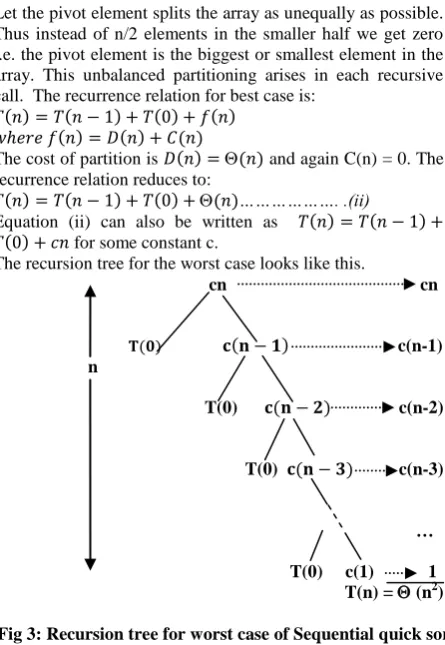
Let the pivot element splits the array as unequally as possible. Thus instead of n/2 elements in the smaller half we get zero i.e. the pivot element is the biggest or smallest element in the array. This unbalanced partitioning arises in each recursive call. The recurrence relation for best case is:

The cost of partition is and again C(n) = 0. The recurrence relation reduces to:

………. .(ii)

Equation (ii) can also be written as

for some constant c.

The recursion tree for the worst case looks like this.

cn cn

c(n-1) n

T(0) c(n-2)

T(0) c(n-3)

…

T(0) c(1) 1

T(n) = (n2₎

Fig 3: Recursion tree for worst case of Sequential quick sort algorithm

Therefore, the running time is : T(n) = (n2

).

2.1.3

Average Case

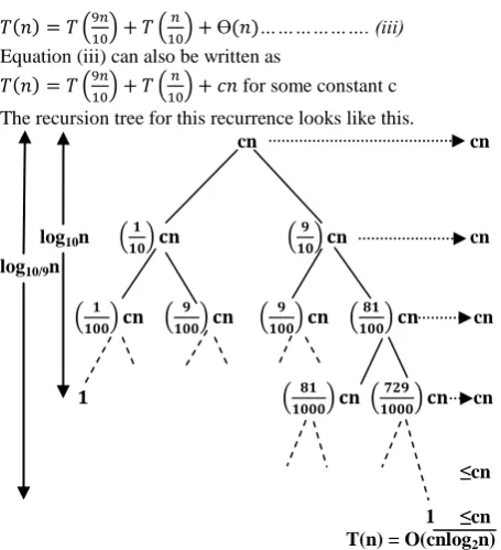
The average-case running time [8] of quick sort is much closer to the best case than to the worst case. Let the partitioning algorithm always produces a 9-to-1 proportional split, which seems quite unbalanced. The recurrence relation seems to be:

Values< Pivot

Pivot Values> pivot Initial Step

Pivot Values>Pivot

Recursive Step Values< New

Pivot

New Pivot

Ө ………. (iii) Equation (iii) can also be written as

for some constant c The recursion tree for this recurrence looks like this.

cn cn

log10n n cn

log10/9n

cn

cn

≤cn

1 ≤cn

T(n) = O(cnlog2n)

Fig 4: Recursion tree for Average case of Sequential quick sort algorithm

Each level of the tree has cost cn, until a boundary condition is reached at depth log10 n, and each level have cost at most

cn. The recursion terminates at depth log10/9 n =log2n/log210=

(log n). The total cost is therefore (nlogn). Thus, with a 9-to-1 proportional split at every level of recursion, which is quite unbalanced, quick sort runs in (nlogn) time, asymptotically the same as the splitting in best case. Even a 99-to-1 split yields an (nlogn) running time.

2.1.4

Total number of comparisons in parallel

quick sort

3.

PARALLEL SORTING

ALGORITHMS

With the advent of parallel processing, parallel sorting has become an important area for algorithm research. A large number of parallel sorting algorithms have been proposed [4]. Most parallel sorting algorithms can be placed into one of two rough categories: merge based sorts and partition-based sorts. Merge-based sorts consist of multiple merge stages across processors, and perform well only with a small number of processors. When the number of processors utilized gets large, the overhead of scheduling and synchronization also increased, which reduces the speedup. Partition-based sorts consist of two phases: partitioning the data set into smaller subsets such that all elements in one subset are no greater than any element in another, and sorting each subset in parallel. The performance of partition-based sorts primarily depends on how well the data can be evenly partitioned into smaller ordered subsets. It appears to be a difficult problem to find pivots that partition the data to be sorted into ordered subsets of equal size without sorting the data first. The basic result [14] is that initial data splitting limits the speedup to a maximum, i.e. about 5 or 6, regardless of how many processors are used. The ability to partition the data evenly into ordered subsets is essential for partition-based sorts.

Parallel sorting algorithms are required in order to speed up the data processing. The parallel implementation of the quick sort algorithm based on divide and conquer approach increases its speed, but fastest sorting is not always guaranteed in cases of poor load balancing of the concurrent tasks. Several optimization techniques are suggested in order to increase the efficiency of the parallel implementation of the quick sort algorithm based on ideas used for parallel implementation of a variety of sorting algorithms [11, 12]. The current trends of hardware development and innovations are oriented towards extensive usage of high-performance computations based on multicomputer and multiprocessor computer systems. Grid and cloud computing also pose the requirement for distributed data processing [2].

Here two parallel sorting algorithms are considered for analysis i.e. Parallel quick sort and Hyperquicksort.

3.1

Parallel quick sort

Not only quick sort is considered to be a better performing sorting algorithm but it is also considered to be one of reliable algorithm which can be parallelized. The key feature of Parallel Quicksort is parallel partitioning of the data [13]. The parallel generalization of the quick sort algorithm [4] may be obtained in the simplest way for a network of processing elements. The topology adapted by network is a D-dimensional hypercube (i.e. number of processing elements p=2D_{). Let the initial data is distributed among the processors}

in blocks of the same size of n/p data values. The resulting location of blocks must correspond to each of the hypercube processors. A possible method to execute the first iteration of the parallel method is as follows [3]:

• Select the pivot element from the subsequence and broadcast it to all the processors

• Subdivide the data block available on each processor into two parts using the pivot element;

• Pairs of processors are formed, for which the bit representation of the numbers differs only in D position. After pairing, the exchange of the data among these processors takes place. As a result of these data transmissions, the parts of the blocks with the data values smaller than pivot element must appear on the processors having bit position D equal to 0. The processors with the bit position D is equal to 1 must collect correspondingly all the data values exceeding the value of the pivot element.

3.1.1

Basic implementation steps [4]

(a) (b) (c)

(d) (e)

Fig 5: 5(a) specifies that one processor broadcast initial pivot to all processors. 5(b) each processor in the upper half swaps with a partner in the lower half. 5(c) specifies recursion on each half. 5(d) shows the swapping among partners in each half. In 5(e) each process uses quick sort to sort elements locally.

3.1.2 Pseudo code of Parallel quick sort algorithm

2. Select the pivot element randomly on first processor P0 and

broadcast it to each processor. 3. Perform global sort

3.1 Locally in each processor, divide the data into two sets according to the pivot (smaller or larger)

3.2 Split the processors into two groups and exchange data pair wise between them so that all processors in one group get data less than the pivot and the others get data larger than the pivot.

4. Repeat 3.1 - 3.2 recursively for each half.

5. Each processor sorts the items it has, using quick sort.

3.1.3 Complexity Analysis

Let the size of input is ’n’ and the number of processing elements taken to be ‘p’.

Total running time of parallel quick sort:

Total number of comparisons in parallel quick sort:

Speedup achieved over sequential quick sort:

3.2

Hyperquicksort

Start where parallel quick sort ends. As the speedup achieved by the parallel quick sort algorithm [11] is constrained by the time taken to perform the initial partitioning. During initial partitioning all the processors are not active. Hyperquicksort is the quick sort algorithm developed for hypercube interconnection networks, but it can be used on any message-passing system having number of processing elements in power of 2.

The main difference between hyperquicksort and parallel quick sort consists in the method of choosing the pivot element. The average element of some block is chosen as the pivot element (generally, on the first processor of the computer system). The pivot element is selected in such a way that it appears to be closer to the real mean value of the sorted sub sequence than any other arbitrarily chosen value.

In hyperquicksort each process sorts its sub list by using the most efficient sequential algorithm i.e. sequential quick sort. It helps in meeting the first requirement of sorting. To meet the second requirement, processes must exchange values by using a communication-efficient parallel algorithm to generate the final solution from the partial solutions. To keep ordering the values in the course of computations, the processors carry out the operation of merging the parts of blocks obtained after splitting.

The effect of splitting and merging operation [12] is to divide a hypercube of sorted list of values into two hypercubes so that each processor has a sorted list of values, and the largest value in the lower hypercube is less than the smallest value in the upper hypercube.

3.2.1

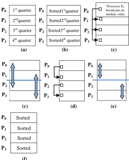
Basic implementation steps

(a) (b) (c)

(c) (d) (e)

(f)

Fig 6: 6(a) specifies that complete sequence is distributed evenly among the processors (which are in power of 2). 6(b) shows that each processor sorts its subsequence by using sequential quick sort. 6(c) Processor P0 broadcasts

P0

P1

P2

P3

Sorted Sorted Sorted Sorted

P0

P1

P2

P3

P0

P1

P2

P3

P0

P1

P2

P3

P2

P1

P0

P3

Sorted1st_quarter

Sorted2nd_quarter

Sorted3rd _quarter

Sorted4th _quarter

P0

P1

P2

P3

1st _quarter

2nd_quarter

3rd _quarter

4th _quarter

P0

P1

P2

P3

Processor P0

broadcasts its medianvalue

< > < > < >

P2

P1

P0

P3

P2

P1

P0

P3

1st quarter

2nd_quarter

3rd _quarter

4th _quarter

< > Unsorted List

< > < > < > < >

P2

P1

P0

P3

P2

P1

P0

P3

P1

P2

P0

P3

Lower Half

its median value. 6(d) Processors will exchange “low”, “high” lists. In 6(e) Processors P0 and P2 broadcast its

median values. In 6(f) each sub half processors exchange “low”, “high” lists. 6(g) show sorted subsequences after exchange and merge steps.

3.2.2 Pseudo code for hyperquicksort

1. Divide the n data values into p equal parts, n/p data values per processor.

2. Each processor sorts the items it has using sequential quick sort.

3. First processor P0 broadcasts its median key K (pivot) to the

rest of the processors in hypercube.

4. Each node separates its data items into two groups: Keys <= K and Keys > K

5. Break up the hypercube into two sub-cubes:

The lower sub-cube consists (node 0 through (2^ (D-1) - 1)) and the upper sub-cube consists (nodes 2^ (D-1) through (2^D - 1)).

5.1 Each node in the lower sub-cube sends its items whose keys are greater than K to its adjacent node in the upper sub-cube.

5.2 Each node in the upper sub-cube sends its items whose keys are less than or equal to K to its adjacent node in the lower sub-cube.

When this step is completed, all items whose keys are less than or equal to K are in the lower sub-cube while all those whose keys are greater than K are in the upper sub-cube. 6. Each node now merges together the group it just received with the one it kept so that its items are one again sorted. 7. Repeat step 3 through 6 on each of the two sub-cubes. This time first processor P0 will correspond to the lowest-number

node in the sub-cube, and the value of D will be one less. 8. Keep repeating steps 3 through 7 until the sub-cubes consist of a single one.

3.2.3 Complexity Analysis

Let the size of input is ’n’ and the number of processing elements taken to be ‘p’.

 Initial quick sort step has time complexity ((n/p) log (n/p))

 Total communication time for log p exchange steps: ((n/p) log p)

 Total communication time for broadcasting the pivot value: (log p)

Total running time of hyperquicksort:

Total number of comparisons in parallel quick sort:

Speedup achieved over sequential quick sort:

4.

CASE STUDY

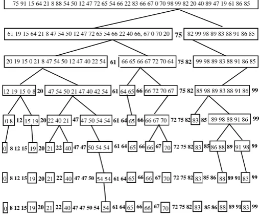
Consider a set S, consisting of 32 unordered data elements given as:

S= {75, 91, 15, 64, 21, 8, 88, 54, 50, 12, 47, 72, 65, 54, 66, 22, 83, 66, 67, 0, 70, 98, 99, 82, 20, 40, 89, 47, 19, 61, 86, 85} This data set is sorted by all the three, above mentioned sorting algorithms viz. sequential quick sort, Parallel quick sort and Hyperquicksort.

4.1

Sorting by Sequential quick sort

Firstly, a pivot element is chosen which divides the data set in two data sets upon which same procedure is performed recursively until we get a sorted sequence. The steps are as follows:

Fig. 7 Recursive sorting by using sequential quick sort

4.2 Sorting by Parallel Quick sort

Perform the steps as mentioned in the pseudo code for parallel quick sort to sort the data set as follows:

(a) (b)

P0

83 66 67 0 70 98 99 82

20 40 89 47 19 61 86 85 50 12 47 72 65 54 66 22

75 91 15 64 21 8 88 54 75 15 64 21 54 66 67 0 70

50 12 47 72 65 54 66 22 20 40 47 19 61

83 98 99 82 91 88

89 86 85

P1

P2

P3

P0

P1

P2

P3 Lower

Half

Upper Half

P0

83 66 67 0 70 98 99 82

20 40 89 47 19 61 86 85 50 12 47 72 65 54 66 22

75 91 15 64 21 8 88 54 75 91 15 64 21 8 88 54

50 12 47 72 65 54 66 22

83 66 67 0 70 98 99 82

20 40 89 47 19 61 86 85

P1

P2

P3

P0

P1

P2

P3

75 91 15 64 21 8 88 54 50 12 47 72 65 54 66 22 83 66 67 0 70 98 99 82 20 40 89 47 19 61 86 85

75

99 98 89 83 88 91 86 85 66 65 66 67 72 70 64

20 19 15 0 21 8 47 54 50 12 47 40 22 54 61 75 82

85 98 89 83 88 91 86 66 72 70 67 75 82

64 65 66 61

47 54 50 21 47 40 42 54

20

15 19

12 20 22 40 2147 47 50 54 5461 64 65 66 66 67 7072 75 82 83 85 89 98 88 91 86

19

8 12 15 20 21 22 40 47 47 50 54 54 61 64 65 66 66 67 ₇₀ 72 75 82 83 85 86 88 89 91 98

8 12 15 19 20 21 22 40 47 47 50 54 5461 64 65 66 ₆₆ 67 70 72 75 82 83 85 86 88 89 91 83

8 12 15 19 20 21 22 40 47 47 50 54 54 61 64 65 66 ₆₆ 67 ₇₀ 72 75 82 83 85 86 88 89 91 83 99 99 99

99 99

0 8 12 15 19 20 21 22 40 46 47 50 54 54 61 64 65 66 66 67 70 72 75 82 83 85 86 88 89 91 98 99 61 19 15 64 21 8 47 54 50 12 47 72 65 54 66 22 40 66, 67 0 70 20 82 99 98 89 83 88 91 86 85

12 19 15 0 8 67

0 8

0

0

(c) (d)

(g) (h)

Fig. 8 Recursive sorting by using Parallel quick sort 8(a) specifies that complete sequence distributed evenly among the processors (which is in power of 2). 8(b) Process P0

chooses and broadcasts randomly chosen pivot value 8(c) specifies exchanging of “lower half” and “upper half” values” 8(d) shows after the exchange step In 8(e) Processors P0 and P2 choose and broadcast randomly

chosen pivots. In 8(f) exchange of values takes place 8(g) Subsequences after the exchange steps. In 8(h) each processor sorts its subsequences by using sequential quick sort.

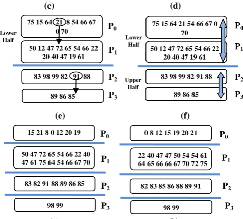
4.3 Sorting by Hyperquicksort

Perform the steps as mentioned in the pseudo code for Hyperquicksort to sort the data set as follows:

(a) (b)

(c) (d)

(e) (f)

(g) (h)

Fig. 9 Recursive sorting by using Hyperquicksort 9(a) specifies that complete sequence distributed evenly among the processors (which are in power of 2). 9(b) each processor sorts its subsequences by using sequential quick sort. 9(c) Processor P0 broadcasts its median value 9(d)

shows that processors will exchange “low”, “high” lists. In 9(e) exchange of values takes place. In 9(f) processors P0

and P2 broadcast median values. 9(g) shows the

communication pattern for second exchange. In 9(h) specifies the sorted subsequences at each processor.

5.

COMPARISON OF RESULTS AND

DISCUSSION

The performance of three algorithms can be analyzed by considering the number of comparisons, average running time and speed up (achieved by parallel sorting algorithms). Table1 shows the number of comparisons performed in all three algorithms and can be implemented in MATLAB 7.0. It shows that the parallel quick sort and hyperquicksort perform better over sequential quick sort, due to the use of parallelism. Between the two parallel sorting algorithms, hyperquicksort perform better and sort the data in less number of comparisons.

Table1. Number of comparisons

Inp

u

t

S

ize

(n

)

S

eq

u

en

tia

l

Q

u

ick

so

rt

Number of comparisons in Parallel Quick sort

Number of comparisons in Hyperquicksort

P=2 P=4 P=8 P=

1

6

P=2 P=4 P=8 P=

1

6

25

2

2

2

.4

129 100 _{75 58 96 56 32 18}

27

1

2

4

5

.4

4

769 644 523 410 512 288 160 ₈₈

29

6

4

0

5

.1

2

4

0

9

7

3

5

8

8

3

0

8

3

2

5

8

6

2

5

6

0

1

4

0

8

768 416

211

3

1

3

1

3

.9

2

2

0

4

8

1

1

8

4

3

6

1

6

3

9

5

1

4

3

6

2

1

2

2

2

8

6

6

5

6

3

5

8

4

1

9

2

0

P0

12 19 20 22 40 47 47 50 54 0 8 15 21 54

61 65 66 72 85 86 89

P1

P2

P3

P0

P2

P3

64 66 67 70 75 82 83 88 91 98 99

P1

19 20 21 22 40 47 47 50 54 54

83 85 86 88 89 91 98 99 0 8 12 15

61 64 65 66 66 67 70 72 75 82

P0

12 19 20 22 40 47 47 50 54 0 8 15 21 54

61 65 66 72 85 86 89

P1

P2

P3

P0

P2

P3

64 66 67 70 75 82 83 88 91 98 99

P1

0 8 15 21 54

12 19 20 22 40 47 47 50 54

64 66 67 70 75 82 83 88 91 98 99

61 65 66 72 85 86 89

P0

0 66 67 70 82 83 98 99

19 20 40 47 61 85 86 89 12 22 47 50 54 65 66 72

8 15 21 54 64 75 88 91 8 15 21 54 64 75 88 91

12 22 47 50 54 65 66 72

0 66 67 70 82 83 98 99

19 20 40 47 61 85 86 89

P1

P2

P3

P0

P1

P2

P3

P0

83 66 67 0 70 98 99 82

20 40 89 47 19 61 86 85 50 12 47 72 65 54 66 22

75 91 15 64 21 8 88 54 8 15 21 54 64 75 88 91

12 22 47 50 54 65 66 72

0 66 67 70 82 83 98 99

19 20 40 47 61 85 86 89

P1

P2

P3

P0

P1

P2

P3

P0

50 47 72 65 54 66 22 40 47 61 75 64 54 66 67 70

15 21 8 0 12 20 19

98 99

P1

P2

P3

P0

P2

P3

83 82 91 88 89 86 85

P1

0 8 12 15 19 20 21

22 40 47 47 50 54 54 61 64 65 66 66 67 70 72 75

82 83 85 86 88 89 91

98 99

P0

50 12 47 72 65 54 66 22 20 40 47 19 61 75 15 64 21 8 54 66 67

0 70

75 15 64 21 54 66 67 0 70

50 12 47 72 65 54 66 22 20 40 47 19 61

83 98 99 82 91 88

89 86 85

P1

P2

P3

P0

P2

P3 Lower

Half

Upper Half

83 98 99 82 91 88

P1

89 86 85

213 1 4 8 0 2 9 .4 4 9 8 3 0 5 9 0 1 1 6 8 1 9 3 1 7 3 7 5 4 5 7 3 4 4 3 0 7 2 0 1 6 3 8 4 8 7 0 4 215 6 8 3 2 1 2 .8 0 4 5 8 7 5 3 4 2 5 9 8 8 3 9 3 2 2 7 3 6 0 4 7 4 2 6 2 1 4 4 1 3 9 2 6 4 7 3 7 2 8 3 8 9 2 217 3 0 9 7 2 3 1 . 4 2 0 9 7 1 5 3 1 9 6 6 0 8 4 1 8 3 5 0 1 9 1 7 0 3 9 6 2 1 1 7 9 6 4 8 6 2 2 5 9 2 3 2 7 6 8 0 1 7 2 0 3 2 219 1 3 8 4 6 4 4 6 .0 9 4 3 7 1 8 5 8 9 1 2 9 0 0 8 3 8 8 6 1 9 7 8 6 4 3 4 6 5 2 4 2 8 8 0 2 7 5 2 5 1 2 1 4 4 1 7 9 2 7 5 3 6 6 4

P : Number of Processing Elements

Figure 10 shows that among the three sorting algorithms hyperquicksort performs better. Between parallel quick sort and hyperquicksort, rate of reduction in number of comparisons is more in hyperquicksort in comparison to parallel quick sort, which results in improved performance.

Fig. 10 Chart for number of comparisons

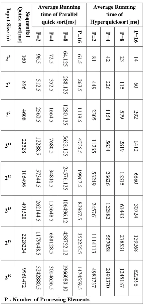
Table 2 shows the average running time of all three algorithms with respect to the increasing number of inputs. Between parallel quick sort and hyperquicksort, the running time of hyperquicksort is less due to better load balancing and selection of pivot element. Also for the same number of processors hyperquicksort has less average running time in comparison to parallel quick sort.

Table2. Average running time

Inp u t S ize (n ) S eq u en tia l Q u ick so rt[m s] Average Running time of Parallel

quick sort[ms]

Average Running time of Hyperquicksort[ms]

P=2 P=4 P=8 P=

1

6

P=2 P=4 P=8 P=

1 6 25 160 9 6 .5 7 2 .5 6 4 .1 2 5 6 1

.5 81 42 23 14

27

896 51

2 .5 3 5 2 .5 2 8 8 .1 2 5 2 6 3 .5

449 226 115 ₆₀

29 4 6 0 8 2 5 6 0 .5 1 6 6 4 .5 1 2 8 0 .1 2 5 1 1 1 9 .5 2 3 0 5 1 1 5 4 579 292 211 2 2 5 2 8 1 2 2 8 8 .5 7 6 8 0 .5 5 6 3 2 .1 2 5 4 7 3 5 .5 1 1 2 6 5 5 6 3 4 2 8 1 9 1 4 1 2 213 1 0 6 4 9 6 5 7 3 4 4 .5 3 4 8 1 6 .5 2 4 5 7 6 .1 2 5 1 9 9 6 7 .5 5 3 2 4 9 2 6 6 2 6 1 3 3 1 5 6 6 6 0 215 4 9 1 5 2 0 2 6 2 1 4 4 .5 1 5 5 6 4 8 .5 1 0 6 4 9 6 .1 2 8 3 9 6 7 .5 2 4 5 7 6 1 1 2 2 8 8 2 6 1 4 4 3 3 0 7 2 4 217 2 2 2 8 2 2 4 1 1 7 9 6 4 8 .5 6 8 8 1 2 8 .5 4 5 8 7 5 2 .1 2 3 5 2 2 5 5 .5 1 1 1 4 1 1 3 5 5 7 0 5 8 2 7 8 5 3 1 1 3 9 2 6 8 219 9 9 6 1 4 7 2 5 2 4 2 8 8 0 .5 3 0 1 4 6 5 6 .5 1 9 6 6 0 8 0 .1 0 1 4 7 4 5 5 9 .5 4 9 8 0 7 3 7 2 4 9 0 3 7 0 1 2 4 5 1 8 7 6 2 2 5 9 6

P : Number of Processing Elements

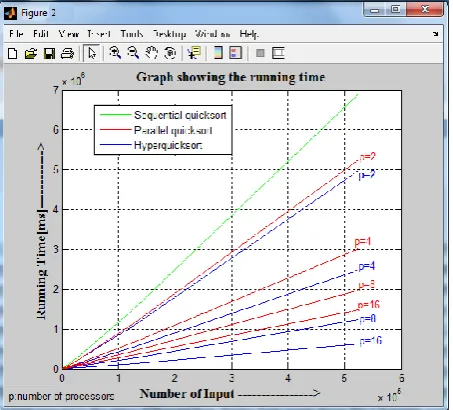
Fig. 11 Comparison chart for average running time

Table 3 specifies the speedup achieved by parallel quick sort over sequential quick sort, which is very poor due to improper load balancing of data values as it is seen in the case study.

Table3. Speedup achieved over sequential quick sort

Num b er o f Pro ce ss in g Elem en ts (p )

Speedup achieved in Parallel quick sort

n = 5 1 2 n = 2 0 4 8 n = 8 1 9 2 n = 3 2 7 6 8 n = 1 3 1 0 7 2 n = 5 2 4 2 8 8 2 1 .7 9 9 6 4 8 5 1 .8 3 3 2 5 8 7 1 .8 5 7 1 2 6 7 1 .8 7 4 9 9 6 4 1 .8 8 8 8 8 8 1 1 .8 9 9 9 9 9 8 4 2 .7 6 8 3 9 8 9 2 .9 3 3 1 4 2 4 3 .0 5 8 7 7 9 6 3 .1 5 7 8 8 4 6 3 .2 3 8 0 9 2 9 3 .3 0 4 3 4 7 3 8 3 .5 9 9 6 4 8 5 3 .9 9 9 9 1 1 2 4 .3 3 3 3 1 1 3 4 .6 1 5 3 7 9 2 4 .8 5 7 1 4 1 5 5 .0 6 6 6 6 6 3 16 4 .1 1 6 1 2 3 3 4 .7 5 7 2 5 9 0 5 .3 3 3 4 6 6 9 5 .8 5 3 6 9 3 4 6 .3 2 5 5 9 0 4 6 .7 5 5 5 5 7 8 32 4 .3 6 8 9 3 7 2 5 .1 7 7 9 9 5 0 5 .9 4 3 2 8 2 1 6 .6 6 6 7 8 2 5 7 .3 5 1 3 8 2 4 8 .0 0 0 0 0 8 2 64 4 .4 7 4 4 6 5 2 5 .3 7 6 8 1 1 5 6 .2 5 6 4 3 1 5 7 .1 1 1 3 3 3 0 7 .9 4 1 6 6 6 9 8 .7 4 8 2 1 8 0

n : Input size

Figure 12 shows the speedup of parallel quick sort with increasing number of inputs i.e. n and processing elements.

Fig. 12 Chart for speedup achieved by parallel quick sort over Sequential quick sort

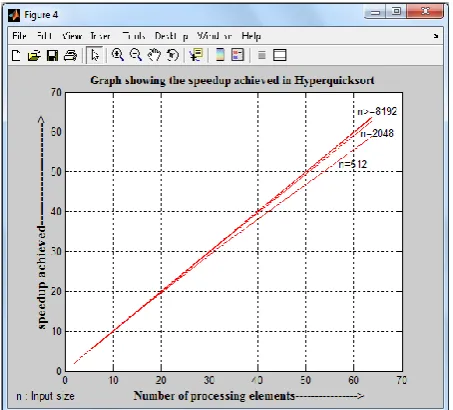
Table 4 specifies the speedup achieved by hyperquicksort over sequential quick sort, that improves in comparison to parallel quick sort due to the good choice of pivot element and even load balancing. All the processing elements are having nearly same number of data values to balance the work performed by all the processors.

Table4. Speedup achieved over sequential quick sort

Num b er o f Pro ce ss in g Elem en ts (p )

Speedup achieved in Hyperquicksort

n = 5 1 2 n = 2 0 4 8 n = 8 1 9 2 n = 3 2 7 6 8 n = 1 3 1 0 7 2 n = 5 2 4 2 8 8 2 1 .9 9 9 1

323 1_.9

9

9

8

225 1_.9

9

9

9

624 1_.9

9

9

9

919 1_.9

9

9

9

982 1_.9

9 9 9 996 4 3 .9 9 3 0 6 7 6 3 .9 9 8 5 8 0 0 3 .9 9 9 6 9 9 5 3 .9 9 9 9 3 4 9 3 .9 9 9 9 8 5 6 3 .9 9 9 9 9 6 8 8 7 .9 5 8 5 4 9 2 7 .9 5 8 5 4 9 2 7 .9 9 8 1 9 7 5 7 .9 9 9 6 0 9 4 7 .9 9 9 9 1 3 8 7 .9 9 9 9 8 0 7 16 1 5 .7 8 0 8 2 2 0 1 5 .9 5 4 6 7 4 0 1 5 .9 9 0 3 9 0 0 1 5 .9 9 7 9 1 7 0 1 5 .9 9 9 5 4 0 0 1 5 .9 9 9 8 9 7 0 32 3 0 .9 2 6 1 7 4 0 3 1 .7 7 4 3 3 0 0 3 1 .9 5 1 9 9 5 0 3 1 .9 8 9 5 8 7 0 3 1 .9 9 7 7 0 2 0 3 1 .9 9 9 4 8 6 0 64 5 9 .0 7 6 9 2 3 0 6 2 .9 2 7 3 7 4 0 6 3 .7 7 0 0 6 0 0 6 3 .9 5 0 0 3 9 0 6 3 .9 8 8 9 7 2 0 6 3 .9 9 7 5 3 3 0

n : Input size

Fig. 13 Chart for speedup achieved by hyperquicksort over Sequential quick sort

6.

CONCLUSION

In this paper, three sorting algorithms are compared successfully. The basis of comparison is the average running time, number of comparisons and speedup achieved by parallel sorting algorithms over sequential quick sort. It is observed that parallel sorting algorithms i.e. parallel quick sort and hyperquicksort performs well in all respects in comparison to sequential quick sort. The better performance is obvious because parallel sorting algorithms take the advantage of parallelism to reduce the waiting time. Between hyperquicksort and parallel quick sort, parallel quick sort does not perform well due to improper load balancing as it selects a random data value as a pivot from one of the subsequence, which results in uneven load distribution. Hyperquicksort selects the median value of subsequence as a pivot for better load distribution. In future, same analysis can be performed with parallel sorting algorithms (parallel quick sort and hyperquicksort) and parallel sorting by regular sampling algorithm (PSRS) for wide variety of MIMD architectures.

7.

REFERENCES

[1] Madhavi Desai, Viral Kapadiya, Performance Study of Efficient Quick Sort and Other Sorting Algorithms for Repeated Data, National Conference on Recent Trends in Engineering & Technology, 13-14 May 2011.

[2] D. E. Knuth, The Art of Computer Programming, Volume 3: Sorting and Searching, Second ed. Boston, MA: Addison-Wesley, 1998.

[3] Grama A., A. Gupta, G. Karypis, V. Kumar, Introduction to Parallel Computing, Addison Wesley, 2003.

[4] M. J. Quinn, Parallel Programming in C with MPI and OpenMP, Tata McGraw Hill Publications, 2003, p. 338.

[5] C.A.R. Hoare, Quick sort, Computer Journal, Vol. 5, 1, 10-15 (1962).

[6] S. S. Skiena, The Algorithm Design Manual, Second Edition, Springer, 2008, p. 129.

[7] Abdulrahman Hamed Almutairi & Abdulrahman Helal Alruwaili, Improving of Quick sort Algorithm performance by Sequential Thread or Parallel Algorithms, Global Journal of Computer Science and Technology Hardware & Computation Volume 12 Issue 10 Version 1.0, 2012.

[8] T.H. Cormen, C.E. Leiserson, R.L. Rivest, Introduction to algorithms, MIT Press 1990.

[9] Akl, S.G., Parallel Sorting Algorithms, Academic Press, Orlando, Florida, 1985.

[10] Borovska P., Synthesis and Analysis of Parallel Algorithms, Technical University of Sofia, 2008, ISBN: 978-954-438-764-4.

[11] Quinn, M.J., Parallel Computing Theory and Practice,

Tata Mcgraw Hill Publications (2002), p. 277.

[12] Akl, S.G., Design and Analysis of Parallel Algorithms, Academic Press, Orlando, Florida, (1985).

[13] P. Heidelberger, A. Norton, and J. T. Robinson. Parallel quicksort using Fetch-and-Add. IEEE Transactions on Computers, 39(1):133–137, January 1990.