Dinkelbach Approach for Solving Interval-valued
Multiobjective Fractional Programming Problems using
Goal Programming
Mousumi Kumar
Department of Mathematics Alipurduar College
Alipurduar Court-736122, West Bengal, India
Bijay Baran Pal
Department of Mathematics
University of Kalyani,
Kalyani-741235, West Bengal, India
ABSTRACT
This paper presents an interval valued goal programming approach for solving multiobjective fractional programming problems. In the model formulation of the problem, the interval-valued system constraints are converted in to equivalent crisp system. The interval valued fractional objective goals are transformed into linear goals by employing the iterative parametric method which is an extension of Dinkelbach approach. In the solution process, the goal achievement function, termed as ‘regret function’, is formulated for minimizing the unwanted deviational variables to achieve the goals in their specified ranges and thereby arriving at most satisfactory solution in the decision making environment.
To illustrate the proposed approach one numerical example is solved.
Keywords
Dinkelbach approach, Fractional Programming, Goal Programming, Interval Arithmetic, Interval Programming.
1.
INTRODUCTION
Goal programming (GP) is an analytical approach used to solve the decision making problems where the target has been assigned to all the objectives. The core of GP lies in the works of Charnes et al., [5], although the actual name first appear in text by Charnes and Cooper [4]. After that this field has been studied by different researches, Lee [19], Ignizio [11], Ignizio and Cavalier [12], Romero [25, 26, 27], and others. In 1995, Schniederjans [28] gives in a bibliography of pre-1995 articles relating to GP and in 2002 Jones and Tamiz [15] give bibliography for the period 1990-2000. A recent textbook by Jones and Tamiz [16], gives a comprehensive overview of the state-of-the-art in goal programming. The main weakness of the conventional GP method is that the aspiration levels of the goals need to be specified precisely in the decision making context. But, in reality, decision makers (DMs) are frequently faced with inexactness. When the coefficients are imprecise then fuzzy programming [1, 32] has been used. On the other hand, if the coefficients are random in nature but their probability distributions are assumed to be known then, the stochastic programming [7, 20] has been used.
Now, in a certain decision situation, it has been realized that parameter values are found to be neither probabilistic nor fuzzy, but they are rather in the form of intervals with certain lower- and upper- bounds.
To overcome such a situation, interval programming (IVP) approach [3, 13, 14, 17], based on interval arithmetic [21], has appeared as a prominent tool for solving decision problems with interval-valued parameter sets.
IVP approaches to decision problems in inexact environment have been deeply studied in [2, 30] in the past. Mainly, two types of methodological aspects are used to solve the IVP problems. The first one is based on the satisficing philosophy of GP and second one is traditional method of optimization. GP approaches [11, 24, 25] to IVP problem have been introduced by Inuguichi and Kume [13] in 1991. The potential use of IVP approach to mobile robot path planning [9] and portfolio selection [10] has been studied in the past. The methodological development made in the past has been surveyed by Oliveira and Antunes [22] in 2007. The application of IVP approach to university management system has been studied by Pal et al., [23] in the recent past. However, the IVP approach and its application to multi objective fractional programming problems (MOFPPs) are yet to be widely circulated in the literature.
In this article, a GP solution approach to MOFPPs with interval valued objectives together with interval valued system constraints is presented. In the model formulation of the problem, the interval valued system constraints are transformed into equivalent crisp system constraints by using the interval inequality relation which was first introduced by Tong in 1994 [31], and further developed by Sengupta et al. [29] in 2001. Then, the target intervals for goal achievement in the interval goal programming approach are determined by considering the individual best and worst objective values of each objective in the decision making horizon. The interval valued objectives with target intervals are transformed into standard goals in the conventional GP formulation by using interval arithmetic operation rule [13] and then introducing under- and over deviational variables to each of them. To avoid the computational complexity of using conventional fractional programming approach [6, 18] to MOFPP, an extended version of Dinkelbach approach [8] is used to convert the fractional objective goals into linear goals to solve the problem by using linear GP methodology.
The proposed approach is illustrated by one numerical example.
2.
PROBLEM FORMULATION
The generic form of an interval valued MOFPP with interval valued system constraints can be stated as:
Find so as to
Maximize:
, r=1,2,…,R
(1) subject to
(2) where and and
(r=1,2,…,R; i=1,2,…,m; j=1,2,…,n) represent the vectors of intervals, and are constant intervals, where L and U stand for the lower and upper bounds of the respective intervals.
It avoid infeasibility, it is customary to assume that,
where S ( ) is the solution region.
Now, some basic concepts of interval arithmetic are discussed in brief in the following Section 3.
3.
THE
BASIC
CONCEPTS
OF
INTERVAL ARITHMETIC
An interval A can be defined an ordered pair as
, where and
are left and right limit of the interval A on the real line R. The midpoint and the width of an interval A can be defined as m[A] and w[A],
where and . Now, a binary operation [21], on the intervals A1= and A2 = are defined as:
A1 (–) A2 = where
The operation (–) and is known as ‘possible subtraction’.
3.1 Definition of necessary deviation in GP
formulation
For the above defined operation, the possible deviation between two intervals sayCrX and Trcan be defined as
for
and for )
(3) where and are two
specified intervals.
Now, using the definition of width of an interval, can be presented as:
,
for ,
for (4)
Here, it is to be followed that the exact upper bound and lower bound of cannot be easily identified in the solution process. To overcome the above difficulty, the goal
expressions of in the conventional forms of goals in GP can be defined and the two forms of goals appear as
(5) where 0 and 0 represent the
under-and over deviational variables associated with the respective goals, and where
Now, in the decision situations the expression of which are regarded as necessary regret intervals, can be obtained in four possible ways as follows [13]:
(i) if and
then, [min ( ), max
(ii) if and
then, [0, max ]
(iii) if and
then, [0, max ]
(iv) if and
then, [min ( ), max
Now, considering the four possible defined values of Dr, the final expression of Dr is obtained as:
(6) where ‘˄’ and ‘˅’ denote the minimum and maximum operators,
i.e. min(a, b) = a ˄ b , max(a, b) =a ˅ b.
Now, the GP formulation of the problem with interval valued fractional objectives defined in Section 2 is described in the Section 4.
4. DETERMINATION OF TARGET
INTERVALS
The r-th objective in (1) can be explicitly expressed as:
(7) Using the interval arithmetic rule [13], the objective in (7) can be presented as:
= , (say), r =1,2,…,R
(8) To determine the target intervals, the best and the worst solutions of the defined interval valued objectives are to be obtained first. For this it is necessary to transfer the interval-valued system constraints into crisp system.
Using the approach introduced by [31] and further studied by [29] for the inequality constraints involving interval coefficients, the crisp equivalent system constraints of the i-th interval constraints in (2) can be written as:
(9) where
and Let, the individual best and worst solutions of the r-th
where
and
Now, from the viewpoint of achieving the objective values within the best and worst decisions, the target intervals can be considered as
, where
Then, incorporating the target intervals, interval valued objectives in (8) can be expressed as [27]:
(10)
5. GOAL PROGRAMMING
FORMULATION
In the GP framework [11], the objectives are transformed into goals by incorporating certain aspiration levels and introducing under-and over-deviational variables to each of them. In the proposed problem, the objectives goals can be constructed from the expression in (10) as:
(11) (12)
where represent under-and
over-deviational variables associated with respective goals and they satisfy the relations,
= 0 and = 0, r = 1,2,…..,R.
It is to be observed that the goals in (11) and (12) are fractional in form. In fractional programming [18], the iterative approach introduced by [8] is adopted in the solution process of the problem.
5.1. Linearization of the Ratio Goals
The fractional form of FrU (X) in the r-th goal expression in (11) can be presented as follows:
Let,
where Nr(X) and Dr(X) are linear functions of
Then the goal expression can be presented as
(13) Now, optimization of the k-th functional goal expression in (13) is equivalent to optimize the functional form:
where is a real number.
Then the linear form of (13) is obtained as
(14) Now, the fractional form of TrL(X) in the r-th goal expression in (11) can be presented as follows:
Now, let
(15)
Proceeding analogous way, the linear parametric form of the goal expression in (12) can be presented as:
(16) Now, it is to be followed that in the solution process, the proposed approach is iterative in nature in the process of solving the problem.
An extended version of the iterative solution procedure in [8] is presented in the following steps.
5.2 The Algorithmic Steps
Step 1: Rename by to represent it at the i-th
solution stage.
Step 2: Set = 0 for i = 1 and r = 1, 2,…, R, R+1,
R+2,…,2R and solve the GP problems in (14) and (16) together with the given system constraints in (9).
Step 3: Let X1 be the solution obtained in the Step 2.
Set i = 2 and determine =Nr(X1)/Dr(X1).
Step 4: Solve the problem in (14) and (16) with the defined .
Step 5: Determine Step 6: Define such that
is a sufficiently smallpositive number.
Step 7: If go to Step 8, otherwise go to Step 10. Step 8: Set i = i + 1.
Step 9: Compute Nr(Xi)/Dr(Xi) and return to the
Step 2.
Step 10: If , terminate the algorithm, and
identify the solution
where is the optimal solution and is the
approximate solution to the problem in the notion of satisficing philosophy in the conventional GP approach.
Note: Regarding convergence of the proposed algorithm, it is to be noted that the executable IVP model involves a number of linear programs in the solution process. Since the solution space is bounded and only the linear programs are involved there in the solution search process, the algorithm always stops after a finite number of iterations.
6. GP MODEL FORMULATION
In a decision making situation, the aim of each of the DMs, is to achieve the goal values within the specified ranges by means of minimizing the possible regrets in terms of the deviational variables involved in the decision situation. In the present decision situation, the goal achievement function is termed as the ‘regret function’, since the regret intervals defined for goal achievement within the specified target intervals are to be minimized to the extent possible in the decision making environment.
Now, in the field of IVP, both the aspects of GP, minsum GP [25] for minimizing the sum of the weighted unwanted deviational variables as well as minmax GP [11] for minimizing the maximum of the deviations, are simultaneously taken into account as a convex combination of them to reach a satisfactory solution within the specified target intervals of the goals.
Then, the regret function appears as [13]:
Minimize:
(17) Taking, ,
the executable GP model of the problem takes the form: Minimize:
and satisfy
together with the system constraints defined in (9),
(18)
where with = 0; r=1,2,…,R and = 0, r = R+1,
R+2,…,2R.
F represents the regret function for goal achievement and where with denote the numerical weights of importance of achieving the goals within the respective target intervals, and .
To demonstrate the feasibility of the approach one numerical example is solved.
7.
NUMERICAL EXAMPLE
Let the interval-valued MOFPP is of the form
Find so as to Maximize F1(X):
Maximize F2(X) :
subject to
(19) Using Section 4 and considering µ = 0.5 (according to the needs and desires of the DM), interval valued system constraints in (19) are converted into crisp form as:
(20)
The objectives in standard form of interval can be presented as:
F1 (X)=
F2 (X)=
(21) Then, following the proposed procedure the individual best and worst solutions of the first objective in (21) are obtained as:
and
The best and worst solutions of the second objective in (21) are obtained as:
and
Now, the target intervals for the defined individual worst and best decisions of the two objectives are successively considered as
[0.30, 0.85] and [0.25, 1.5].
Using interval arithmetic technique, equivalent objective goals can be defined as:
(22)
Then following the above procedure and iterative approach, GP formulation of the problem can be obtained as:
Find so as to Minimize Z
so as to satisfy
subject to the crisp system constraints in (20), and
(23)
where
with
Considering equal weights i.e. w1 = w2 = 1/2 and , the
problem is solved by using linear GP methodology.
In the solution process, taking ε = 0.5 and the Software LINGO (ver. 12.0) solver (the permissible size of instance is 500 variables and 250 constraints) is used to solve the problem iteratively. This model (variable size 11, constraint size 11) is executed in Pentium IV CPU with 2.66 GHz Clock-pulse and 2GB RAM. The required CPU time is approximately 0.001 second.
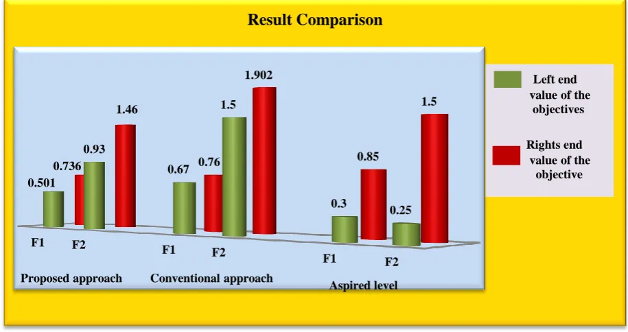
The optimal solution is achieved at the fifth iteration. The resultant decision is
(x1, x2) = (1.3469, 0.7729) with
F1=[0.501, 0.736], F2=[0. 93, 1.46].
The result shows that a satisfactory solution within the specified target intervals is reached in the decision making environment.
Note: It is to be noted that, instead of employing the linearization approach, if the problem of achievement of the fractional goals in (22) together with the system constraints in (20) is directly considered and solved by using the conventional interval GP approach, then the solution is obtained as
(x1, x2) = (0, 2.33) with
F1= [0.67, 0.76], F2 = [1.5, 1.902].
Fig.1: Graphical representation of the achievement of objective values under the proposed approach and the conventional approach
It can easily be followed form the above graph that more acceptable decision is achieved here under the proposed approach than the conventional approach with regard to the achieving the goal values within their specified target intervals.
8. CONCLUSION
The main advantage of the proposed approach is that the computational complexity with the fractional goals does not arise here due to the efficient use iterative approach.
The use of the proposed approach to real-world decision problems is an emerging area for study in future. The proposed approach may be extended to solve the hierarchical decentralized decision problem with interval parameter sets. However, it is hoped that approach presented in this paper will open up a new vistas of research on interval programming for its actual implementation of real-world problem in inexact environment.
9. ACKNOWLEDGMENTS
The authors are grateful to the anonymous referees for their valuable suggestions which have led to improve the presentation of the paper. The author Mousumi Kumar, is also grateful to the University grant Commission (UGC), New Delhi, India, for providing financial support to carry out the research work.
10.
REFERENCES
[1] Bellman, R. E., Zadeh, L.A. 1973. Decision making in a fuzzy environment. Management Sciences, vol. 17, pp. B141-B164.
[2] Bitran, G. R. 1980. Linear multiobjective problems with interval coefficients. Management Science. vol. 26, pp. 694-706,
[3] Chanas, S., Kuchta, D. 1996. Multiobjective programming in optimization of interval objective functions – a generalized approach. European Journal of Operational
Research. vol. 94, pp. 594-598.
[4] Charnes, A., Cooper, W. W. 1961. Management Models and Industrial Applications of Linear Programming, Vol. I and II. Wiley, New York.
[5] Charnes, A., Cooper, W. W. and Ferguson, R.
1955. Optimal estimation of executive compensation by linear programming. Management Science. vol.1, pp.138-151.
[6] Craven, B. D. 1988. Fractional Programming. Heldermann Verlag, Berlin.
[7] Dempster, M. A. H. 1980. Stochastic Programming, Academic Press.
[8] Dinkelbach, W. 1967. On Nonlinear Fractional Programming. Management Science. vol. 13, pp. 492 – 498.
[9] Ida, M. 2000. Interval multiobjective programming and mobile robot path planning”. In: Mohammadian, M., Mohammadian, M., (Eds). New Frontiers in Computational Intelligence and it’s Applications. IOS Press, pp. 313-322.
[10]Ida, M. 2003. Portfolio selection problem interval coefficients. Applied Mathematics Letters, vol. 16, pp 709-713.
[11]Ignizio, J. P. 1976. Goal Programming and Extensions, Lexington, Massachusetts, D. C. Health.
[12]Ignizio, J. P., Cavalier, T. M. 1994. Linear Programming. Prentice Hall, New Jersey.
[13]Inuiguchi, M. Kume, Y. 1991. Goal programming problems with interval coefficients and target intervals. European Journal of Operational Research. vol. 52, pp. 345-361.
[14]Ishibuchi, H., Thanaka, H. 1990. Multiobjective programming in optimization of interval objective
F1 F2
F1 F2
F1 F2
0.501
0.93
0.67
1.5
0.3
0.25 0.736
1.46
0.76
1.902
0.85
1.5
Result Comparison
Left end value of the objectives
Rights end value of the objective
Proposed approach Conventional approach
Aspired level
function. European Journal of Operational Research. vol. 48, 219-225.
[15]Jones, D. F., Tamiz, M. 2010. Practical Goal programming. Springer Books.
[16]Jones, D. F., Tamiz, M. 2002. Goal programming in the period 1990-2000, in Multiple Criteria Optimization: State of the art annotated bibliographic surveys, M. Ehrgott and X. Gandibleux (Eds.), pp. 129-170. Kluwer Pub.
[17]Kerfortt, R. B. 1989. Interval mathematical techniques for control theory computation. K. Bowers and J. Lund (eds.), Computation and Control, Proceedings of the Bozeman Conference, vol. 20 of Progression Systems and Control Theory, Birkhauser, Boston, MA, pp.169-178.
[18]Kornbluth, J. S. H., Steuer, R. E. 1981. Multiple Objective Linear Fractional Programming. Management Science, vol. 27, pp. 1024 – 1039.
[19]Lee, S. M. 1972. Goal Programming for Decision Analysis. Auerbach Pub., Philadelphia.
[20]Liu, B. 2002. Theory and Practice of Uncertain Programming. Physica-Verlag, Heidelberg.
[21]Moore, R. E. 1966. Interval analysis, Prentice-Hall, New Jersey,.
[22]Oliveira, C. and Anunes, C. H. 2007. Multiple objective linear programming models with interval coefficients – an illustrated overview. European Journal of Operational Research. vol. 118, pp. 1434-1463.
[23]Pal, B. B., Kumar, M., and Sen, S. 2012. A priority–based goal programming method for solving academic personnel planning problems with interval–valued resource goals in
university management system. International Journal of Applied Management System. vol. 4, No. 3, pp. 284-312.
[24]Romero, C. 1986. A survey of generalized goal programming. European Journal of Operational Research, vol. 25, pp. 183–191.
[25]Romero, C. 1991. Handbook of Critical Issues in Goal Programming. Pergamon Press, Oxford.
[26]Romero, C. 2001. Extended Lexicographic Goal Programming: A Unifying Approach. Omega, vol. 29, pp. 63 – 71.
[27]Romero, C. 2004. A General Structure of Achievement Function For a Goal Programming Model. European Journal of Operational Research. vol. 153, pp. 675 – 686.
[28]Schniederjans, M. J. 1995. Goal Programming: Methodology and Applications. Kluwer, Boston.
[29]Sengupta, A., Pal, T. K. and Chakraborty, D. 2001. Interpretation of inequality constraints involving interval coefficients and a solution to interval linear programming. Fuzzy Sets and Systems, vol. 119, pp. 129-138.
[30]Steuer, R. E. 1981. Algorithm for linear programming problems with interval objectives function coefficients. Management Science. vol. 26, pp. 333 – 348.
[31]Tong, S. 1994. Interval number and fuzzy number linear programming. Fuzzy Sets and Systems, vol. 66, pp. 301– 306.