http://dx.doi.org/10.4236/ajcm.2015.52010
Comparison of Fixed Point Methods and
Krylov Subspace Methods Solving
Convection-Diffusion Equations
Xijian Wang
School of Mathematics and Computational Science, Wuyi University, Jiangmen, China Email: [email protected]
Received 2 March 2015; accepted 5 June 2015; published 9 June 2015
Copyright © 2015 by author and Scientific Research Publishing Inc.
This work is licensed under the Creative Commons Attribution International License (CC BY). http://creativecommons.org/licenses/by/4.0/
Abstract
The paper first introduces two-dimensional convection-diffusion equation with boundary value condition, later uses the finite difference method to discretize the equation and analyzes positive definite, diagonally dominant and symmetric properties of the discretization matrix. Finally, the paper uses fixed point methods and Krylov subspace methods to solve the linear system and com-pare the convergence speed of these two methods.
Keywords
Finite Difference Method, Convection-Diffusion Equation, Discretization Matrix, Iterative Method, Convergence Speed
1. Introduction
In the case of a linear system Ax=b, the two main classes of iterative methods are the stationary iterative me-thods (fixed point meme-thods) [1]-[3], and the more general Krylov subspace methods [4]-[13]. When these two classical iterative methods suffer from slow convergence for problems which arise from typical applications such as fluid dynamics or electronic device simulation, preconditioning [14]-[16] is a key ingredient for the success of the convergent process.
The goal of this paper is to find an efficient iterative method combined with preconditioning for the solution of the linear system Ax=b which is related to the following two-dimensional boundary value problem (BVP)
( ) ( )
( )
( )
2 2
2
2 2 , , , 0,1
0, , .
u u u u
f x y x y
x y
x y
u x y
γ
− ∂ +∂ + ∂ −∂ = ∈ Ω =
∂ ∂ ∂ ∂
= ∈ ∂Ω
(1)
For parameter γ =0,16, 64, we use finite difference method to discretize the Equation (1). Take n+2 points in both the x- and y-direction and number the related degrees of freedom first left-right and next bottom-
top. Now, we take n=32, thus the grid size 1 1 2 1 33
x y h
n
∆ = ∆ = = =
+ − . For γ =0, the convection term
equals to 0, using central difference method to the diffusion term, we get the discretization matrix of the Equa-tion (1) 0 0 0 0 0 0
4 1 0 0
1 4 1
, 0 0 .
1 4 1
0 0 0 1 4
B I O O
I B I
A O O B
I B I
O O O I B
− − − − − − = = − − − − − − (2)
For
γ =
16
, the diffusion term use a central difference and for the convection term use central differences scheme as the following:(
)
( )1 ( )1 ( 1) ( 1) ( )1 ( )1 ( 1) ( 1)2 2
2 2
, ,
2 2
ij ij
i j i j i j i j i j i j i j i j ij ij
u u u u u u u u u u
f x y
h h
h h γ
+ − + − + − + − + − − + − −
= − + + −
(3)
we obtain the discretization matrix of the Equation (1)
(
)
(
)
(
)
(
)
(
)
(
)
1 1
1 1 1
1
1 1 1
1 1 1 1 1 , 1 1 1
B c I O O
c I B c I
A O O
c I B c I
O O O c I B
− + − − − + = − − − + − − (4) where
(
)
(
)
(
)
(
)
(
)
(
)
1 1 1 1 1 1 1 14 1 0 0
1 4 1
8
, .
0 0
2 33
1 4 1
0 0 0 1 4
c c c h B c c c c γ − − − + − − = = = − + − − − +
For γ =64, the diffusion term use a central difference and for the convection term use upwind differences scheme as the following:
(
)
( )1 ( )1 ( 1) ( 1) ( )1 ( 1)2 2
2 2
, i j ij i j i j ij i j ij i j i j ij ,
ij ij
u u u u u u u u u u
f x y
h h
h h γ
+ − + − + − + − − − + −
= − + + −
(5)
we obtain the discretization matrix of the Equation (1)
(
)
(
)
(
)
2 1 2 1 2 2 1 2 1 1 , 1B c I O O
I B c I
A O O
I B c I
O O O I B
where
(
)
(
)
(
)
2 1 2 2 2 1 2 1 24 2 1 0 0
1 4 2 1
64
0 0 , .
33
1 4 2 1
0 0 0 1 4 2
c
c c
B c h
c c c c γ + − − + + − = = = − + + − − + +
2. Properties of the Discretization Matrix
In this section, we would first compute the eigenvalues of the discretization matrices A0, A1 and A2 of Equ-ation (1), later analyze positive definite, diagonally dominant and symmetric properties of these matrices.
2.1. Eigenvalues
Using MATLAB, the eigenvalues of the discretization matrices A0, A1 and A2 of Equation (1) are the fol-lowing:
( )
( )
( )
0 , 21 , 1
2 , 2 2
π π
4 2 cos cos ,
1 1
π π
4 2 1 cos cos , , 1, 2, , .
1 1
π π
4 2 2 1 cos cos ,
1 1 p q p q p q p q A n n p q
A c p q n
n n
p q
A c c
n n λ λ λ = + + + + = + − + = + + = + + + + + +
(7)
2.2. Definite Positiveness
Matrix A is positive definite if and only if the symmetric part of Ai.e.
T
2 S
A A
A = + is positive definite. Since
( )
002 0
, 0,
, 1,
1 , 2,
2 i S
A i
A A i
c A i = = = + =
we have all the eigenvalues of
T
2 i i A +A
(i = 0, 1, 2) are the following:
( )
(
)
( )
2
0 , 1
, 2 2 2 0 1 , π π
4 2 1 cos cos 0, 0,1,
1 1
, 1, 2, , .
π π
1 1 4 2 1 cos cos 0, 2,
2 2 1 1
p q i S p q
p q
p q
A c i
n n
A p q n
c c p q
A c i
n n
λ λ
λ
= + − + > =
+ + = =
+ = + + − + > =
+ +
(8)
Therefore
( )
i SA (i = 0, 1, 2) is positive definite, which means the discretization matrices A0, A1 and A2
of Equation (1) are positive definite.
2.3. Diagonal Dominance
( )
(
) (
)
( )
(
)
( )
0 1 , 1 22 2 4 , ;
2 1 2 1 4 , ;
2 1 2 4 2 , .
jj ij
n
ij jj ij
i j i
jj ij
a A a
a c c a A a
c c a A a
≠ = + = = = ≤ + + − = = = + + = + = =
∑
Therefore, the discretization matrices A0, A1 and A2 of Equation (1) are diagonally dominant.
2.4. Symmetriness
It is easy to see that only A0 is symmetric.
3. Stationary Iteration Methods and Krylov Subspace Methods
The goal of this section is to find an efficient iterative method for the solution of the linear system , 0,1, 2
i
A x=b i= . Since A ii
(
=0,1, 2)
are positive definite and diagonally dominant, we would use fixed point methods and Krylov subspace methods. In this section, first find the suitable convergence tolerance, later use numerical experiments to compare the convergence speed of various iteration methods.3.1. Convergence Tolerance
Without loss of generality, take b=Ax x*, * =
(
1,1,,1)
T, convergence tolerance3 1 2 2 10 i b A
δ = −−
⋅ and assume
that 2
2 i Ax b
b δ
−
≤ , then
(
)
1 1
* 2 2 2 2
1 2 1 3
2 2 2 2
2
10 .
i i i
i
x x A Ax b A Ax b
Ax b
b A b A
b δ − − − − − − = ⋅ − ≤ ⋅ − − = ⋅ ⋅ ≤ ⋅ ⋅ =
In order to achieve xi−x* 2≤10−3 in the numerical experiments, we would set convergence tolerance 3 1 2 2 10 i b A
δ = −−
⋅ .
3.2. Numerical Experiments
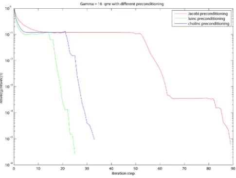
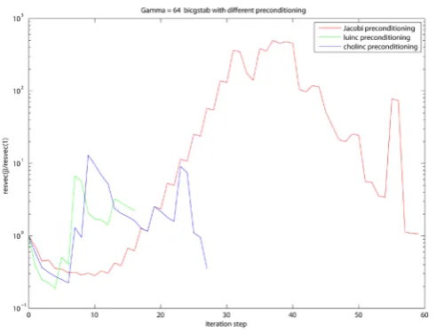
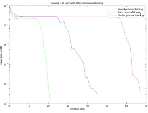
Computational results using fixed point methods such as Jacobi, Gauss-Seidel, SOR etc. and projection methods such as PCG, BICG, BICGSTAB, CGS, GMRES and QMR are listed out in figures (Figures 1-21), for all three different
γ
values(
γ
=0,16, 64)
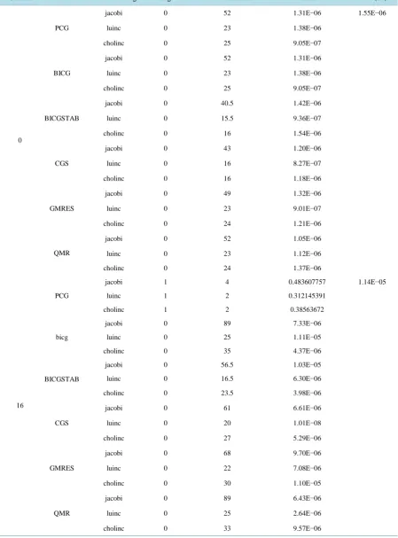
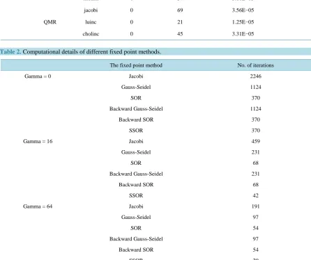
. The projection methods are performed with different preconditioning me-thods such as Jacobi preconditioning, luinc and cholinc preconditioning.The tables (Table 1andTable 2) containing relevant computational details are also given below.
4. Conclusions
From the figures (Figures 1-21) and tables (Table 1andTable 2), we obtain the following conclusions:
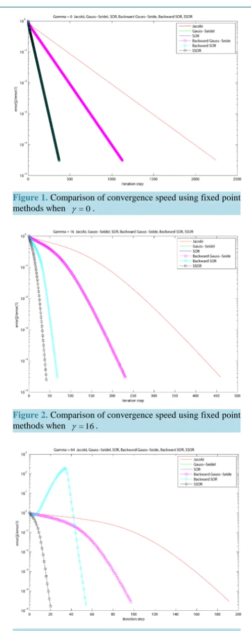
• The convergence speeds of SOR, Backward SOR and SSOR are faster than that of GS and Backward GS; while GS and Backward GS are faster than Jacobi;
• If matrix A is symmetric
(
γ
=0)
, the convergence speeds of SOR, Backward SOR and SSOR are the same; otherwise(
γ
=16, 64)
, SSOR is faster than Backward SOR and SOR;• The convergence speeds of SOR and Backward SOR are the same, also for GS and Backward GS;
• FromTable 2, the iteration steps and the time for all fixed point methods of the case in which γ =64 are less than the case in which γ =16, and also the case in which γ=16 are less than the case in which γ =0;
Figure 1. Comparison of convergence speed using fixed point methods when γ = 0.
Figure 2. Comparison of convergence speed using fixed point methods when γ = 16.
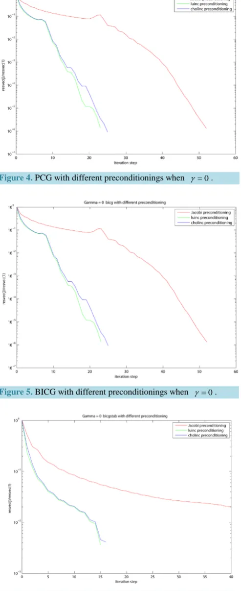
[image:5.595.203.426.502.687.2]Figure 4. PCG with different preconditionings when γ = 0.
Figure 5. BICG with different preconditionings when γ = 0.
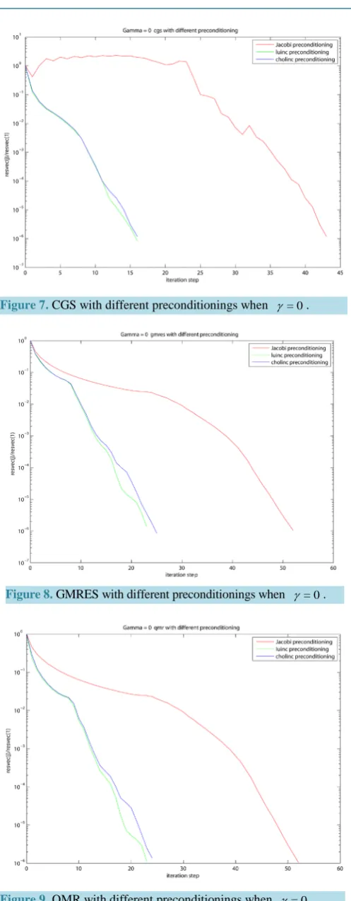
Figure 7. CGS with different preconditionings when γ = 0.
Figure 8. GMRES with different preconditionings when γ = 0.
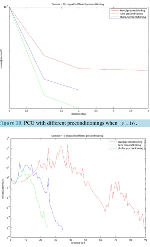
Figure 10. PCG with different preconditionings when γ = 16.
Figure 11. BICG with different preconditionings when γ = 16.
Figure 13. CGS with different preconditionings when γ = 16.
Figure 14. GMRES with different preconditionings when γ = 16.
Figure 16. PCG with different preconditionings when γ= 64.
Figure 17. Bicg with different preconditionings when γ= 64.
[image:10.595.192.438.515.703.2]Figure 19. CGS with different preconditionings when γ= 64.
Figure 20. GMRES with different preconditionings when γ= 64.
[image:11.595.193.437.516.703.2]Table 1. Computational details of different projection methods with different preconditioning.
Gamma Function Preconditioning flag No. of iterations Relres Delta (tol)
0
PCG
jacobi 0 52 1.31E−06 1.55E−06
luinc 0 23 1.38E−06
cholinc 0 25 9.05E−07
BICG
jacobi 0 52 1.31E−06
luinc 0 23 1.38E−06
cholinc 0 25 9.05E−07
BICGSTAB
jacobi 0 40.5 1.42E−06
luinc 0 15.5 9.36E−07
cholinc 0 16 1.54E−06
CGS
jacobi 0 43 1.20E−06
luinc 0 16 8.27E−07
cholinc 0 16 1.18E−06
GMRES
jacobi 0 49 1.32E−06
luinc 0 23 9.01E−07
cholinc 0 24 1.21E−06
QMR
jacobi 0 52 1.05E−06
luinc 0 23 1.12E−06
cholinc 0 24 1.37E−06
16
PCG
jacobi 1 4 0.483607757 1.14E−05
luinc 1 2 0.312145391
cholinc 1 2 0.38563672
bicg
jacobi 0 89 7.33E−06
luinc 0 25 1.11E−05
cholinc 0 35 4.37E−06
BICGSTAB
jacobi 0 56.5 1.03E−05
luinc 0 16.5 6.30E−06
cholinc 0 23.5 3.98E−06
CGS
jacobi 0 61 6.61E−06
luinc 0 20 1.01E−08
cholinc 0 27 5.29E−06
GMRES
jacobi 0 68 9.70E−06
luinc 0 22 7.08E−06
cholinc 0 30 1.10E−05
QMR
jacobi 0 89 6.43E−06
luinc 0 25 2.64E−06
Continued
64
PCG
jacobi 1 1 0.710978037 4.13E−05
luinc 1 1 0.547110057
cholinc 1 1 0.660611555
BICG
jacobi 0 70 3.15E−05
luinc 0 21 1.21E−05
cholinc 0 44 3.47E−05
BICGSTAB
jacobi 0 59.5 2.12E−05
luinc 0 16.5 5.27E−06
cholinc 0 27.5 1.60E−05
CGS
jacobi 1 87 0.000123357
luinc 0 19 6.36E−07
cholinc 0 35 3.14E−06
GMRES
jacobi 0 63 2.66E−05
luinc 0 19 2.50E−05
cholinc 0 37 3.11E−05
QMR
jacobi 0 69 3.56E−05
luinc 0 21 1.25E−05
[image:13.595.87.534.333.707.2]cholinc 0 45 3.31E−05
Table 2. Computational details of different fixed point methods.
The fixed point method No. of iterations
Gamma = 0 Jacobi 2246
Gauss-Seidel 1124
SOR 370
Backward Gauss-Seidel 1124
Backward SOR 370
SSOR 370
Gamma = 16 Jacobi 459
Gauss-Seidel 231
SOR 68
Backward Gauss-Seidel 231
Backward SOR 68
SSOR 42
Gamma = 64 Jacobi 191
Gauss-Seidel 97
SOR 54
Backward Gauss-Seidel 97
Backward SOR 54
tral difference method;
• The convergence speed of the six projection methods including PCG, BICG, BICGSTAB, CGS, GMRES and QMR under luinc preconditioning are faster than under cholinc preconditioning, while under cholinc pre-conditioning are faster than Jacobi prepre-conditioning;
• The six projection methods under Jacobi, luinc and cholinc are convergent when γ =0, however, for
16, 64
γ = , the PCG method are not convergent and also the CGS method under Jacobi preconditioning are not convergent when γ =64.
Acknowledgements
I thank the editor and the referee for their comments. I would like to express deep gratitude to my supervisor Prof. Dr. Mark A. Peletier whose guidance and support were crucial for the successful completion of this paper. This work was completed with the financial support of Foundation of Guangdong Educational Committee (2014KQNCX161, 2014KQNCX162).
References
[1] Saad, Y. (2003) Iterative Methods for Sparse Linear Systems. Siam, Bangkok.
http://dx.doi.org/10.1137/1.9780898718003
[2] Varga, R.S. (2009) Matrix Iterative Analysis. Volume 27, Springer Science & Business Media, Heidelberger. [3] Young, D.M. (2014) Iterative Solution of Large Linear Systems. Elsevier, Amsterdam.
[4] Lanczos, C. (1952) Solution of Systems of Linear Equations by Minimized Iterations. Journal of Research of the Na-tional Bureau of Standards, 49, 33-53. http://dx.doi.org/10.6028/jres.049.006
[5] Hestenes, M.R. and Stiefel, E. (1952) Methods of Conjugate Gradients for Solving Linear Systems.
[6] Walker, H.F. (1988) Implementation of the GMRES Method Using Householder Transformations. SIAM Journal on Scientific and Statistical Computing, 9, 152-163. http://dx.doi.org/10.1137/0909010
[7] Sonneveld, P. (1989) CGS, a Fast Lanczos-Type Solver for Nonsymmetric Linear Systems. SIAM Journal on Scientific and Statistical Computing, 10, 36-52. http://dx.doi.org/10.1137/0910004
[8] Freund, R.W. and Nachtigal, N.M. (1991) QMR: A Quasi-Minimal Residual Method for Non-Hermitian Linear Sys-tems. Numerische Mathematik, 60, 315-339. http://dx.doi.org/10.1007/BF01385726
[9] van der Vorst, H.A. (1992) Bi-CGSTAB: A Fast and Smoothly Converging Variant of Bi-CG for the Solution of Non-symmetric Linear Systems. SIAM Journal on Scientific and Statistical Computing, 13, 631-644.
http://dx.doi.org/10.1137/0913035
[10] Brezinski, C., Zaglia, M.R. and Sadok, H. (1992) A Breakdown-Free Lanczos Type Algorithm for Solving Linear Sys- tems. Numerische Mathematik, 63, 29-38. http://dx.doi.org/10.1007/BF01385846
[11] Chan, T.F., Gallopoulos, E., Simoncini, V., Szeto, T. and Tong, C.H. (1994) A Quasi-Minimal Residual Variant of the Bi-CGSTAB Algorithm for Nonsymmetric Systems. SIAM Journal on Scientific Computing, 15, 338-347.
http://dx.doi.org/10.1137/0915023
[12] Gutknecht, M.H. (1992) A Completed Theory of the Unsymmetric Lanczos Process and Related Algorithms, Part I.
SIAM Journal on Matrix Analysis and Applications, 13, 594-639. http://dx.doi.org/10.1137/0613037
[13] Gutknecht, M.H. (1994) A Completed Theory of the Unsymmetric Lanczos Process and Related Algorithms. Part II.
SIAM Journal on Matrix Analysis and Applications, 15, 15-58. http://dx.doi.org/10.1137/S0895479890188803
[14] Eisenstat, S.C. (1981) Efficient Implementation of a Class of Preconditioned Conjugate Gradient Methods. SIAM Jour- nal on Scientific and Statistical Computing, 2, 1-4. http://dx.doi.org/10.1137/0902001
[15] Meijerink, J.V. and van der Vorst, H.A. (1977) An Iterative Solution Method for Linear Systems of Which the Coeffi-cient Matrix Is a Symmetric M-Matrix. Mathematics of Computation, 31, 148-162.
[16] Ortega, J.M. (1988) Efficient Implementations of Certain Iterative Methods. SIAM Journal on Scientific and Statistical Computing, 9, 882-891. http://dx.doi.org/10.1137/0909060