Munich Personal RePEc Archive
The future development of living
standards of the retirees in Belgium. [:]
an application of the static
microsimulation model station
Dekkers, gijs
Centre for Social Policy (CSB)
1999
Online at
https://mpra.ub.uni-muenchen.de/36005/
The future development of living standards of the retirees in
Belgium
.
An application of the STAtic microsimulaTION model STATION
Gijs J.M. Dekkers
Centre for Social Policy (CSB)
Antwerp University UFSIA
Abstract: This paper develops a dynamic microsimulation model with static ageing to
assess the consequences of the assumptions and hypothesis of the Federal Planning
Bureau on the prospective adequacy of pensions. A less technical and shorter version
of this text was published as Gijs Dekkers, 2000, L‟évolution du pouvoir d‟achat des
retraités: Une application du modèle de microsimulation STATION. in: Pestieau, P.,
L. Gevers, V. Ginsburgh, E. Schokkaert, B. Cantillon, Réflexions sur l’avenir de nos
Retraites, Garant, Leuven/Apeldoorn (also available in Dutch).
JEL-codes: J14, D31, I32
Chapter 1. Introduction and problem formulation.
1.1. Introduction.
1.2. A birds-eye view on the Belgian pension system.
1.3. Demographic trends in Belgium.
1.4. What is microsimulation?
1.4.1. Dynamic microsimulation.
1.4.2. Static microsimulation.
Chapter 2. Antwerp STATION.
2.1. The first key technique: reweighting to incorporate ageing.
2.2. The first key technique: reweighting to incorporate changing family structures.
2.3. The second key structure: uprating.
2.3.1. Uprating: what assumptions are made?
2.3.2. The link between wages and pension benefits.
2.3.3. Introducing a wage-barrier in the determination of the level of the
pension benefit.
2.3.4. Contributions.
2.4. Static microsimulation in practice: pitfalls and solutions.
2.4.1. The first pitfall: structural deviation of the weighting factors.
2.4.2. The second pitfall: empty cells.
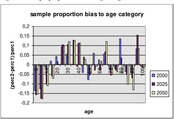
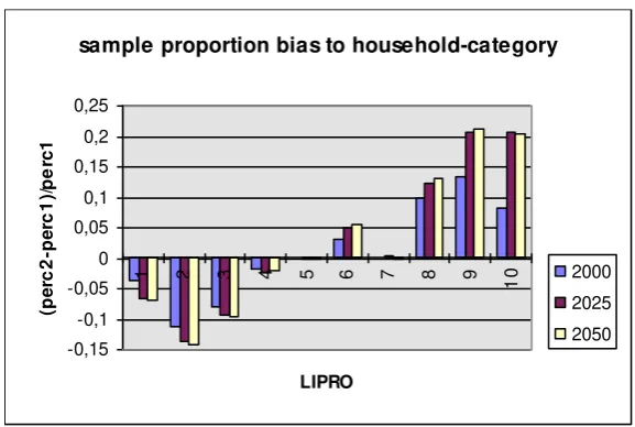
2.4.3. The third pitfall: sample bias.
2.4.4. The fourth pitfall: households versus individuals.
2.5. Conclusion.
Chapter 3: Simulation results.
3.1. Introduction.
3.2. Average incomes.
3.3. Poverty and income inequality.
3.4. Changing the point of view: what would happen if certain measures were not
Chapter 4: Criticisms, discussion and conclusion.
4.1. Criticisms and discussion.
Chapter 1. Introduction and problem formulation
.1.1. Introduction.
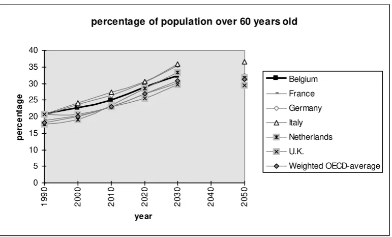
As is the case in most western countries, the Belgian population is greying. As
an illustration, consider the following figure, where the number of individuals over 60
years old is expressed as a percentage of the population (source: World Bank, 1994, P.
[image:6.595.91.477.259.492.2]349).
Figure 1: Percentage of population over 60 years old.
percentage of population over 60 years old
0 5 10 15 20 25 30 35 40
1
9
9
0
2
0
0
0
2
0
1
0
2
0
2
0
2
0
3
0
2
0
4
0
2
0
5
0
year
p
e
rc
e
n
ta
g
e
Belgium France Germany Italy Netherlands U.K.
Weighted OECD-average
The percentage of retirees is relatively high in Belgium in 1990, but is growing
somewhat slower than in the other countries, so that it ends up somewhere in the
middle in 2050. So, the rate of ageing may be moderate if compared to countries such
as the Netherlands and Italy, but it remains significant in itself. As could be expected,
the consequences of such important population shifts have been explored thoroughly,
not only its macroeconomic consequences, but (and probably even primarily) its
consequences for the financial sustainability of public pension systems and health care
services. (for instance, see World Bank, 1994, Creedy (ed.) 1995 and Bos (ed), 1993,
Jackson, 1992, Jackson, 1998, Lesthaeghe, Meeusen, Vandewalle, 1998, Quinn,
1997). As far as pensions are concerned, various empirical models have been
developed with the aim of giving policy makers insight to the process of ageing and
its consequences for the financial sustainability of pensions. (For instance, see,
Heerwaarden, Eikelboon, den Heijer, 1996, for the Netherlands, Bengtsson and Kruse,
1993 for Sweden, De Callatay and Turtelboom, 1996, and (in a broader context)
d‟Alcantara and Wardenier, 1997, Aaron, 1977, Kingsland, 1982).
The model which has recently been developed at the Belgian Federal Planning
Bureau (Festjens, 1997), referred to as PENSION, fits in this rich tradition. As is the
cast in most of the above models, it disentangles several subgroups within the ageing
population and shows what will happen to the contribution rates if the average pension benefits are kept constant, or vice versa. It is a model of the „flow or vintage type‟, where annual flows of 7 types of retirees (Festjens, idem, p. 6) are taken as a basis for a „mechanical‟ calculation of the pension benefits (Festjens, idem, p. 5). The author refer to the model PENSION as a submodule of the general model MALTESE
(Festjens, idem, p.7), thereby emphasising the tight links between PENSION and the
other models developed at the Bureau. An important characteristic of the model is that
it does not extrapolate historical information, since this information can not be a
reference for future generations of retirees (Festjens, idem, p.4 paragraph B). To a
certain extent, this is certainly true: specific circumstances (such as the second
World-War or the economic heydays of the sixties) cause the socio-economic profile of
generations to be different from other generations. However, it seems the most
efficient to use all information available today, including historical information.
Moreover, the model uses simulation results from macroeconomic models (HERMES
and MALTESE) and demographic projections as input factors. These models combine
historical information with scientific knowledge about identities and causal relations.
Consequently, historical information does enter the pension models, though this link
is indirectly. Lastly, and this is specific to the questions the model to be presented in
this study tries to answer, the only information we have on the future distribution on
income is the current distribution of income. Up to today, theory does not provide us
with specific unambiguous empirical identities or causal relations which we can use to
simulate the income distribution in a future point in time, without using the current
distribution of income as a point of departure. We therefore have no choice but to use
the historical information on the distribution of income.
The simulation results of these kinds of vintage-like models as PENSION is,
usually take the form of time-series, showing the simulated future development of,
or not ageing will become a (financing) problem in the future, and give them an idea
on what actions they could take in order to preserve financial sustainability. Useful as
these models are, they fail to show the redistributive impact of the pension system and
the effect of ageing on this redistribution (and related variables, such as poverty). In
other words, these models show what the policy makers can do to keep the pension
system payable, if would they decide that action is required. But they do not show
what the effect of these potential measures on the distribution of pension-benefits or
the poverty rates among the retirees will be. It is however clear that when we consider
the future welfare of the retirees, it is not enough only to look at the development of
the average pension benefit. Other information, such as the distribution of
(pension)income around the mean, poverty rates and such should be taken into
account1.
To overcome this lack of information concerning income distribution,
microsimulation models have been developed. What microsimulation models exactly
are will be explained in depth in the next paragraph, but let us just highlight the basic
difference with the models we just came to mention. This difference is that the point
of departure of these models is the population (or subgroups within the population) as
a whole, where the point of departure of microsimulation models is the individual
itself.
In this study, the effect of ageing on pension income inequality, poverty and
welfare of the retirees will be considered. It this respect, the model which forms the
basis of this study, the microsimulation model STATION, can be seen as being
complementary to the PENSION-model of the Belgian Federal Planning Bureau, since
it uses some of the assumptions of this model to show the consequences on the
poverty rates, income distribution and future development of welfare of the retirees.
So, this study concentrates on what effect potential policy measures (or the not-taking
of these policy measures) will have on the future income distribution, poverty and welfare development of the retirees. The „income-side‟ of the pension system is under consideration only to the extent that it is strictly necessary, so for questions as „will
1Barry (1990, p.2) describes the link between welfare and (redistributional) justice as „inextricably‟.
the pension system remain payable in the future‟, the reader is referred to other
literature, notably Festjens, 1997, and de Callatay et. al, 1996.
The above discussion can be summarised in the following problem definition:
what is the effect of ageing on the development of pension-benefits, the inequality of
pension-benefits and poverty and how will these circumstances change as a result of
some assumptions and policy measures used in the PENSION-model by the Federal
Planning Bureau?
This study starts by a brief discussion of the Belgian pension system. Next, we
will turn our attention to microsimulation models: what is microsimulation? What
kind of techniques are associated with microsimulation and what are their advantages
and disadvantages? As a third step, the static microsimulation model STATION will
be explained in depth and the fourth step will then be the presentation and discussion
of the simulation results. Finally, conclusions will be drawn.
Before proceeding, a last introductory remark must be made. In order to
facilitate co-operation with researchers from other universities, an internet-homepage
has been made. The address of this STATION-homepage is
http://www.ufsia.ac.be/~gdekkers/station/index.htm. This homepage offers those who know the required passwords the possibility to download the simulation results (i.e.
the weighting variables), which can then be used in other empirical studies. Of course,
a more extensive technical description of how to use the simulation results, is
provided as well.
1.2. A birds-eye view on the Belgian pension system.
The Belgian pension system consists of three layers of which the first one is
the most important. The first layer consists of three separate state-wide pension
systems for employees, civil servants and self-employed. The benefits paid out to
retirees in a certain year are financed by contributions of the working generations (a
system widely known as a Pay-As-You-go System or PAYG), though the government
contributes heavily as well2. For all three systems, the pension benefit is equal to 60 or
2
75%3 of a certain wage base, times the relative length of the career (expressed in 45th
for males and 40th for females, though this latter figure is now gradually being
adjusted). The wage-base is either the career-long average wage (or profit) for
employees and self-employed, or the average wage of only the last five years of the
career for civil servants. Given a certain minimal length of career, the system provides
a minimum pension benefit.
These separate pension schemes for employees, self-employed and civil servants are supplemented by a system of „guaranteed income for retirees‟, a welfare-scheme providing those retirees who never had a career or a career of insufficient length with
a minimal and means-tested pension benefit.
The second layer of the Belgian pension system consists of semi-collective
additional pension schemes, organized on the firm level by pension funds. Though
this second layer is rapidly gaining importance, the relative number of
pension-receiving households is still rather limited (see Dekkers, 1998, table 2 and Neyt, 1993,
p. 362). The third level consists of individual pension schemes and life-insurances.
These last two pension benefits are voluntary, based on capital funding instead of
Pay-As-You-Go and are complementary to the nation-wide first-layer pension system.
The microsimulation model STATION, which is the raison d’être of this text,
concentrates on the first layer of the Belgian pension system.
1.3. Demographic trends in Belgium
Next, let us glance at the demographical situation of Belgium for a moment.
This paragraph, which draws heavily on chapters 2 and 3 of the book by Lesthaege,
Meeusen and Vandewalle (idem, 1998), will briefly discuss both past and
expected-future demographic trends in Belgium.
The recent „demographic history‟ of Belgium is characterized by two important demographic transitions, of which the second is the most relevant in this
context. The first demographic transition took place in the nineteenth century and
started with a decrease of the mortality rate (as a result of medical improvements and
increasing knowledge on hygiene). This was followed by a decrease of the fertility
3
rate, resulting from urbanisation and secularisation. Moreover, the average age of
marriage started to decrease, and the relative number of celibate individuals rose.
The second demographic roughly started in the second half of the fifties. This
transition was triggered by changing social values, among other things on the role of
the family in society and the emancipation of women. During the first half of the
sixties, and probably partially resulting from the fact that economic growth rates were
very high, the average age of marriage decreased even further, and so did the average
number of years between marriage and having the first child. Consequently, fertility
reached a maximum, resulting in the so-called „baby-boom‟. However, mainly as a
result from the introduction of the contraceptive pill, combined with increasing
economic independence of women (and therefore higher „opportunity costs‟ of
maternity), the fertility rate again decreased rapidly. This effect was strengthened by a delay of marriage and parentage. As a result, a „baby-bust‟ started in the second half of the seventies and continued during the eighties. The fertility rate was 2.25 in 1970,
which is above replacement-rate, but then decreased to 1.69 in 1980 and 1.55 in 1996
and 1996 (idem, 1998, table 2.6, p. 40).
Demographic behavioural changes like the ones described hitherto change
demographic structures and the effects of this are of a typical long-term nature. These
changes therefore form a basis for projections of the future. Additionally, assumptions
on the future course of some key variables make it possible to distinguish simulation
variants. In this text, only one variant will be discussed, since it forms the basis of the
simulations of the Federal Planning Bureau and, consequently, our own simulations4.
The key assumptions underlying the projections of scenario A of the National Institute
of Statistics and the Federal Planning Bureau are, first of all, that the life expectancy
at birth (which is now 80 years for men and women taken together) will increase to
82.1 for males and 88.1 for females. Secondly, the migration balance (which has a
positive balance of 10,000 immigrants per year in 1995) will decrease to 3,000 in
2050. Thirdly, fertility increases rapidly from 1,55 in 1995 to 1.75 in 2010 and
remains stable thereafter.
4
It must however be noted that Lesthaeghe et. al. think that the assumed future
recovery of the fertility rate is too high, and that the decrease of the proportion of
individuals younger than 20 is therefore underestimated.
The described historical developments, together with the assumptions, result in
some main demographic trends. First of all, the rate of ageing will be quite strong
between 2010 and 2030. It will not only be caused by an increase of the proportion of retirees („greying‟), but by a decrease of the proportion of young individuals as well. Thirdly, immigration can prevent the population to decrease from a certain point on,
but its negative effect on ageing will be small, if any.
Of course, the changes in demographic behaviour as mentioned above, have
their consequences for the household structure in Belgium. Based on projections by
Boulanger et. al. (idem, up to 2011), the following trends for four broad
age-categories can be mentioned. As far as children and young individuals up to 20 years
of age are considered, the most important trend is that the proportion of children
living in households where there is only one parent, or where parents cohabit, will
increase. Young adults (between 20 and 34) will tend to remain living with their
parents more often. Moreover, the proportion of married individuals, especially with
children, in this age-category will decrease. From the beginning of the eighties on, the
proportion of young adults living alone has been increasing. This trend will persist,
though at a lower speed as more and more individuals will cohabit.
For older adults (say between 40 and 65), the trend that the proportion of
married parents decreases, emerges as well. This effect is however less strong for
individuals of 55 and older, since more young adults postpone forming their own
household and remain living with their parents. As a result of an increasing
probability of divorce, the proportion of older adults who live alone, increases.
Lastly, the trends for the retirees must be described. Two main trends emerge:
first of all, the life expectancy of couples increases strongly, so the average age of
losing ones partner increases as well. Secondly, the proportion of retirees living with
relatives will decrease, as will be the case with the proportion of retirees living in
institutions.
Here ends the description of the demographic situation of Belgium, now and in
will be answered. The following step will then be the presentation and description of
the microsimulation model STATION and its simulation results.
1.4. What is microsimulation?
Socio-economic models can be subdivided according to the level on which
they apply. First of all, there are macroeconomic models. These models simulate
entire countries or even groups of countries. Secondly, there are meso-economic
models which concentrate on the simulation of one or more branches of industry
within a country. The third category of socio-economic models has emerged the most
recently and take (groups of) individuals as the point of departure. The models in this
category are called microsimulation models and aim at evaluating the effect of various
economic- and social changes on the distribution of certain characteristics for different
groups of individuals. Mostly , the goal of microsimulation models is to analyse the
changes in the poverty rates and the distribution of income over groups in the
population, resulting from external changes, such as demographic changes, economic
development and policy changes.
The way which microsimulation models work can best be explained by
rephrasing it to a problem common in econometrics and sociometrics, namely that of
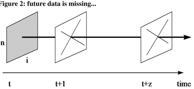
missing data analysis. Suppose we have a cross-sectional dataset at time t, consisting
of n variables describing i individuals. Suppose furthermore a dataset of n variables
and j individuals at the future time point t+z, z>0, which can be considered as
[image:13.595.93.428.562.716.2]consisting completely of missings, as shown in figure 2:
Figure 2: future data is missing...
Now microsimulation models basically are tools to fill in the missing datasets
missings can be filled in by two general methods: cold-deck imputation and hot-deck
imputation (for an introduction to these techniques, see Kalton, 1983). These two
methods form the basis of the division of microsimulation models in static5 - and
dynamic microsimulation models. Both types will be discussed briefly below.
1.4.1. Dynamic microsimulation.
Dynamic microsimulation basically fills in the missing datasets by using
hot-deck imputation. Taking the cross-sectional dataset in time t as the point of departure,
every individual in this dataset faces certain probabilities of a change in each of the n
variables which describe him or her. Whether or not the value of one descriptive
variable actually changes is determined by a Monte-Carlo process. Let us consider a
stylised example: consider an individual of a certain age. Given this age, he or she
faces a certain risk of mortality denoted by d. Now for our individual, a random
number between 0 and 1 is drawn from an uniform distribution. If the resulting
number is below the mortality risk d (which can in turn be a function of other
variables) then the individual is considered dead at t+1. If not, he remains alive, with
the result that his age is increased with one. Likewise, our living individual faces a
certain probability (technically speaking) of becoming married, having a child, finding
or losing a job, and so forth. The number of variables which can be altered between
subsequent points in time depends entirely on how much information on transition
probabilities is available to the constructor of the model.
With dynamic microsimulation, the life history as well as earnings history of
individuals belonging to different groups within the sample can be simulated. The
modeller has relative freedom in what to add to the model. An important advantage is
that it is possible to define individual stock-variables, adding up past values of the
flow-type. For instance, the lifetime-income of an individual can be kept track of by
adding up past (discounted) annual values of income over the whole lifetime of the
individual. As a result, the effect of socio-economic policy measures can be expressed
5
Indeed, this distinction between „static‟ and „dynamic‟ microsimulation models is somewhat
confusing, since both types of models are dynamic in the sense that they are time-dependent. So, a
formally better (but less appealing) description could have been „statically time-dependent‟ and
in terms of „lifetime-income‟ instead of annual income of various groups and generations of individuals, since the latter can be expected to be biased in the sense
that the redistributive effect of a certain measure is generally overestimated when
expressed in terms of annual income. (Nelissen, 1995, and Harding, 1993). As will
become clear when discussing static microsimulation models, this is one of the more
important advantages of dynamic- over static microsimulation models. However,
dynamic microsimulation models have disadvantages too: first of all, they are
generally very large in terms of source code, they usually are very complex and take a
long time to develop. As a result the costs of maintenance are high, and it takes quite
some time to introduce new researchers to the technical details of the model.
Moreover, their use and trustworthiness is restricted to the availability of trustworthy
transition data. Lastly, dynamic microsimulation models make extensive use of
computer recourses, though this is becoming less important due to the rapid
development of computers. Moreover, as opposed to static models, dynamic
microsimulation models do not allow the immediate jump from today to -say- 2020
without having to simulate all the intermediate years. An application of dynamic
microsimulation on the pension system in the Netherlands is Dekkers et. al, 1995.
1.4.2. Static Microsimulation.
In her 1993-book on microsimulation, Harding (Harding, 1993, p.19, see also
Harding, 1996, p.3) describes two key techniques involved in the static ageing of a
dataset. The first one is to reweigh the sample, whereas the second key technique is
referred to as uprating. Both techniques are used in STATION, the static model under
consideration here. However, as it is the most fundamental technique of the two - and
very typical for static microsimulation models, this section will concentrate on the
first key technique: the reweighting of the dataset.
As said in paragraph 1.3, the reweighting-technique of static microsimulation
is basically cold-deck imputation of missing variables. The vast majority of
cross-sectional datasets contain a weighting variable which gives the individual more or less
importance (i.e. a greater or smaller weight) in the sample in order to make the sample
microsimulation models include a notion of „time‟, being reflected in changing (demographic)
more representative for the whole population, for instance by neutralising the effect of
selective nonresponse. The technique of static microsimulation boils down to
adjusting these individual weights to let the dataset in the base year t meet
descriptions of the future population, which are exogenous from the point of view of
the model.
Suppose for instance that a 1992-dataset consists of a certain percentage of
female individuals aged between 15 and 19 and suppose that we know from
demographic projections that this proportion will decrease by 8.5% between 1992 and 2020. Then the „2020-proportion‟ of women can be formed by multiplying the weight variable of the women in this age group by (1-0.085)=0.915. Note that the weight
factors of other categories must be adjusted upwards to neutralise the effect of this
decreasing proportion of young women on the weighted size of the dataset as a whole.
The basic difference between static and dynamic microsimulation models is
that the actual individual data remain unchanged in the case of static microsimulation
modelling; only the weight factor is altered corresponding to the future situation. In
dynamic models, by contrast, the weight variable remains unchanged but the actual
individual information is changed according to individual transition risks and using a
Monte-Carlo process. In reality, however, the difference is often less clear, since both
techniques can be used in the same model.
The disadvantages of dynamic models are the advantages of static
microsimulation models: the latter are technically simple (relative to dynamic models,
that is), though less intuitive and less CPU-demanding6 than dynamic models. This
efficiency is increased further by the fact that, one can form the „2020-dataset‟ in one
step, without having to simulate all the intermediate years first. Moreover, one can use
the simulation results in other empirical research without having any technical
knowledge on the model itself. In the case of STATION, the simulated
weight-transformators can be downloaded from the homepage.
A drawback of static models is its lack of flexibility, compared to dynamic
microsimulation models. Moreover -and this is probably the most serious drawback of
static microsimulation models- the fact that simulation periods in time can be skipped reveals that the model does not have a „memory‟. To make this more clear, let us
6
return to the example of how to calculate the lifetime income (i.e. the income which
an individual earns over his or hers whole life) in a dynamic microsimulation model,
and consider whether or not this could also be done in a static microsimulation model.
In order to construct the lifetime income of an individual, the annual income of this
individual in each year of his or her life is added up. So, a new variable is created
when an individual is born and increased each year, until the individual deceases . Is
this possible in a static model? No, simply because the individual does not get born,
gets older and deceases in a static model. The individual data remains unchanged:
only the weights change. Moreover -again as opposed to dynamic microsimulation-
the simulation results for a certain year x do not influence the simulation results of
another year y, since these simulation results are both directly calculated from the
base-data set. Consequently, the adding up of annual income -even if it would be
meaningful- is not possible.
This discussion of the drawbacks of static microsimulation models ends the
first part of this text. In this part, an introductory overview of microsimulation and the
two types of microsimulation models was given. Both static and dynamic
microsimulation models have their advantages and disadvantages, which are to a
certain extent mutually exclusive. In the second part of the text, which now follows,
the static microsimulation model STATION, developed by the author at the Centre for
Social Policy (Centrum voor Sociaal Beleid or CSB) of Antwerp University (UFSIA),
will be presented and discussed.
Chapter 2. Antwerp STATION.
When the need for a microsimulation model emerged, there was consensus
among the CSB-researchers that this model should meet a number of demands, of
which a short development period was not the least important one. Another thing was
that there was doubt about the availability of enough transition data for a dynamic
model. Moreover, a crucial demand was that the model should make it possible to be
linked to other models of the CSB.
For these and other reasons, it was decided to build a static microsimulation
model, named STATION (from STAtic microsimulaTION, indeed: the name of the
every day to commute between home and work). STATION describes the future
development of the Belgian population starting in 1992 and allowing simulation of
every year up to 2050. It aims at analysing the effects of demographic change (notably
greying) on the Belgian social security system, and it is designed to be a
complementary part of MISIM, the microsimulation model describing the Belgian
social security- and tax-system, developed at the Centre for Social Policy. This model
MISIM (MIcroSImulatieModel) is a static microsimulation model for direct taxes and
benefits7. The relation between MISIM and STATION is best described by quoting
Merz: „Static microsimulation naturally is connected with the time period of the cross-section data [which, in the case of MISIM is 1992, G.D.] Temporal
extrapolation to actualize the data or to forecast the sample into the future, called ageing of the sample, however, is available in more recent static [microsimulation models, G.D.]‟ (Merz, 1994, p.6). It is this last sentence which describes the role of STATION.
The model STATION is written in SAS and consists of one general program
and various submodules, which take the form of SAS-macros, generally with the
projection-year as the only argument. The first submodule modifies the age- and
gender structure of the 1992-dataset. The second submodule changes the distribution
of the family-type to the future situation. This body of the model is completed by a
number of SAS-macros, one of which deals with the intrapolation of the exogenous
projection data. Other macros upgrade variables which reflecting economic growth,
indexation and such. Moreover, additional and separate macros derive a number of
dependent informative variables, such as poverty rates, income inequalities and so
forth.
The model STATION transforms weight variables, which are then applied to
the 1992-wave of the Socio-Economic Panel of the Centre for Social Policy. The
SEP-panel data set started in 1985 and continued in 1988, 1992 and recently 1997. The
1992-wave of the SEP consists of 3821 households, of which 2285 are Flemish and
1177 are Walloon (Cantillon, et. al., 1993, p.7). Due to its size and as a result of
weighting techniques, aiming to correct for selective attrition and non-response, the
panel can be considered representative for the population (idem, p.7 and Proost, et.al.,
7
1996). So, every household in the dataset has an accompanying weighting variable.
The dataset consists of a number of individual- and household characteristics.
Monthly available income (of which the most important are net labour income and
various sources of social security income) is gathered on the household level as well
as on the individual level. Moreover, some household-specific income sources (such
as housing grants) are also asked for. Lastly, and less relevant in this study, there is an extensive list of individual‟s consumption pattern, their attitude towards their income, and so forth.
The simulation results of the core modules of the model STATION are
basically growth rates, which can be used to transform the household population
weighting variable of the Socio-Economic Panel. These latter results will be presented
in the third chapter of this study. The transformation of sample weights can be done
on the individual - or the household level. For any future year between 1992 and 2050,
the model generates a list containing the following variables for every individual.
1. INDnum: an unique number for every individual in the 1992-dataset.
2. LIPRO: family-classification of individual INDnum.
3. weegL: individual transformation according to the future age-distribution
(module 1).
4. weegG: individual transformation according to the future
LIPRO-distribution (module 2).
For every future year and for every individual in the 1992-dataset, the two
transformation variables are generated by the model.
How can these simulation results be used? Suppose for instance that one
wants to see how the income distribution of a certain subset of the Socio-Economic
Panel changes between 1992 and, say, 2030. Or -which is possible as well- suppose
that one wants to know how the estimation results of a certain behavioural relation
change between 1992 and 2030. How can this be done? First of all, one derives the
unique individual identification number INDnum out of other variables in the
SEP-dataset8. Next, the above-mentioned list of transformation variables for the year 2030
must be combined with the SEP-dataset, using INDnum as the merging-variable.
Thirdly, the household-weighting factor must be multiplied with one (or more) of the
8
transformation variables, depending on whether the variable is on the individual- or
household level. The resulting dataset is the 1992-dataset, but then transformed to
2030 which can then be used to answer the questions stated above. If one wants to -as
will be done in this study- one can uprate any monetary variable in the weighted
dataset, using whatever assumptions one wants, provided that one does not want to
use individual stock-variables, as explained earlier. In the presentation of the
simulation results in paragraphs 2.1 and 2.2, uprating will be ignored, since the effect
of reweighting will be shown by looking at some key demographic variables. In
paragraph 2.3, the upgrading technique will be discussed in depth. The third chapter
will entirely be devoted to the presentation and discussion of simulation results which
combine reweighting and upgrading.
Before considering the model as well as the simulation results which stem
from the weight-transformation process and upgrading, a final note must be made on
the simulation years for simulation results will be presented further in this study: even
though this will only be presented for the years 1995, 2000, 2005 and so forth, up to
2050, the model is capable to simulate all in-between years as well.
Next , the two modules which form STATION will be discussed in more
depth. To see their effect on the data, figures describing the situation in the original
dataset of 1992 will be compared to simulation results for the years 1995, 2000, 2005
and up to 2050. These simulation results will only be the result of the transformation
of individual sample weights in the dataset and corresponding changes in income
variables will therefore not be presented yet, since they lack realism.
2.1. The first key technique: reweighting to incorporate ageing.
The first submodule adjusts the age-gender structure of the 1992-dataset to the
combined age-gender projections provided by the Belgian National Institute for
Statistics and the Federal Planning Bureau (source: basic scenario of the
Bevolkingsvooruitzichten 1992-2050). These projections show the future proportion of every age group - and gender combination in the dataset, relative to the
1992-proportions. The projections range from 1995 up to 2050 with five-year jumps (e.g.
1995, 2000, 2005, 2010...) and are indices with 1992 as the base year (or equal to
well, these projections were intrapolated. Thus, the first submodule ables us to modify
the age-gender structure of the 1992 dataset to every future year between 1995 and
2050. This modification is done by simply multiplying the weight factors with the
corresponding future indexes.
As the Belgian population ages, one of the general effects of this first module
is that the weighting factor of older individuals increases ceteris paribus, whereas the
weighting factor of younger individuals decreases, as could be expected. This can be
seen by looking at figure 3.
Figure 3: Age-distribution.
0 2 4 6 8 10
age
%
0 5
10 15
20 25
30 35
40 45
50 55
60 65
70 75
80 85
90 95
100
1992 2020 2050
age-distribution
1992-2020-2050
Ageing is caused by two independent effects. First of all, if a cohort is much larger
than the succeeding cohorts, this cohort will have a disproportional influence on the
age-structure of the entire population. This is sometimes compared with a piglet
swallowed by a snake (Becker, 1994, p.212, Lesthaeghe et. al, 1998, p. 61). After
being swallowed, the piglet is pushed through the snake, while slowly being digested.
Analogous to this, the babyboom-cohort moves right along the horizontal axis, while
its size decreases as a result of mortality. The second -and probably more important-
cause of the ageing of the population is the extension of the life-expectancy, resulting
from technological, medical and economical development. The effect of the longer
life-expectancy is reflected by the decrease of the size of the cohorts, or the speed of
digestion of the piglet by the snake. This effect does not come forward from the above
graph very clearly, but it can still be seen that the difference in the size of the „bump‟
goes by, the negative effect of the mortality rate on the size of the bump decreases,
showing the effect of decreasing mortality rates.
It could seem from figure 3 that there is virtually no difference between the
proportions of the oldest age-groups at the three points in time. Concluding that the
relative size of these oldest groups does not change would be erroneous, since this
change is surpressed by the scale of the y-axis. Figure 4 shows the average growth rate
of the proportions of the age-gender groups over the whole projection period. Here,
the scaling effect is neutralised and the important effect of ageing on the relative sizes
of the oldest age-groups is easily seen.
Figure 4: Average growth rate of the age-gender proportions.
-0.05 0 0.05 0.1 0.15
age
a
v
e
ra
g
e
g
ro
w
th
r
a
te
0 5
10 15
20 25
30 35
40 45
50 55
60 65
70 75
80 85
90 95
100
age-distribution
average grow th rate of age-gender proportions
Figure 4 clearly depicts that, as a result of ageing, the size of the older age-groups will
increase (especially the very-old), whereas the relative size of the younger cohorts
decreases. The turning point lies around the age of 45.
2.2. The first key technique: reweighting to incorporate changing family structures.
In the second submodule, the family structure of the 1992- dataset is altered to
meet family structure projections based on the „realistic scenario‟ of Boulanger, P., A.
Lambert, P. Deboosere and R. Lesthaeghe (la Formation des Familles: étude
Prospective), of which the projection period is from 1996 to 20119. Before proceeding
9
with the explanation of this module, it is important to realise that the distribution by
the family-type LIPRO changes due to the individual ageing as described in paragraph
2.1. as well. For instance, as more older individuals live alone, the number of
one-person households can be expected to increase. From Boulanger et.al., we know what
percentage of the future population will be in what LIPRO-classification, given their age and gender. The model compares the percentage of the „age-gender modified‟ sample with these projected proportions, and transforms the individual weighting
factors to meet these proportions. Consequently, changes in the distribution of
family-type which are independent of the age-gender distribution are imposed on the data. In
other words, this second modules changes the distribution by LIPRO given the
distribution of age and gender.
First of all, we need to know the different types of family which are
distinguished. This classification is known as the LIPRO-classification and consists
of the following entries:
1. Child of a married couple.
2. Child of an unmarried couple.
3. Child of an one-parent family.
4. Single.
5. Married individual without children.
6. Married individual with children.
7. Cohabiting individual without children.
8. Cohabiting individual with children.
9. Head of an one-parent family.
10. Living in the same house as 4, 5 or 6.
11.Others.
The last category (others) a.o. contains individuals living in nursery homes,
psychiatric institutions and other (nonvoluntary) collective forms of cohabitation.
However, these individuals do not occur in the 1992-dataset, so a direct comparison to
the proportions in this dataset with the Boulanger-projections is not possible. To
overcome this problem, the projected proportions have been recalculated, excluding
individuals in every age-gender-category, the projected numbers of individuals in each
age-gender and family-type were derived. Next, the numbers of individuals in the last
category („others‟) were excluded from the dataset, and the proportions were calculated again.
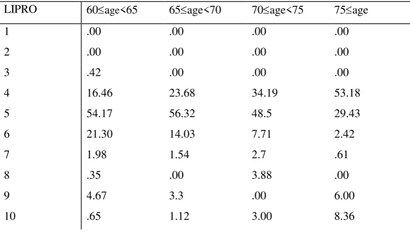
In the following figures, the numbers of individuals in a certain
family-category are represented as a fraction of the total number of individuals in that same
age-category. In other words, these figures representing the probability that an
individual is to be observed in a certain family-type, given that he or she is in a
certain age-category. Taking the percentages to the total numbers of individuals in every age group largely neutralises the effect of ageing, since the first module
transforms the weighting factors for age-groups as a whole. This means that in the
following figures, the changes are mostly due to changing family-type distributions,
and (to a large extend) disregard ageing.
Figure 5 & 6: LIPRO-classification, % age group.
0 20 40 60 80 100
LIPRO
p
e
rc
e
n
t
1 2
3 4
5 6
7 8
9 10
1992 2020 2050
LIPRO: age<20
1992-2020-2050
0 10 20 30 40
LIPRO
p
e
rc
e
n
t
1 2
3 4
5 6
7 8
9 10
1992 2020 2050
LIPRO: 20<=age<30
Figure 7 & 8: LIPRO-classification, % age group. 0 20 40 60 80 LIPRO p e rc e n t 1 2 3 4 5 6 7 8 9 10 1992 2020 2050
LIPRO: 30<=age<40
1992-2020-2050 0 20 40 60 80 LIPRO p e rc e n t 1 2 3 4 5 6 7 8 9 10 1992 2020 2050LIPRO: 40<=age<50
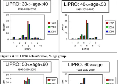
1992-2020-2050Figure 9 & 10: LIPRO-classification, % age group.
0 10 20 30 40 50 LIPRO p e rc e n t 1 2 3 4 5 6 7 8 9 10 1992 2020 2050
LIPRO: 50<=age<60
1992-2020-2050 0 20 40 60 LIPRO p e rc e n t 1 2 3 4 5 6 7 8 9 10 1992 2020 2050LIPRO: 60<=age
1992-2020-2050Remember that the horizontal axis consists of the household-types, of which
the entries are given on page 20. In figure 5, it seems hardly surprising that the vast
majority of the individuals younger than 20 are children of married couples (1), as this
is the most traditional family-form. It is not very surprising either that the importance
of this group is decreasing over time, a decrease which primary occurs in the first half
of the simulation period. It is quite interesting to see that the relative number of
children living in one-parent families (3) is higher than children from unmarried
couples (2). The importance of both categories increases as the relative size of
category 1 decreases. Again, this increase is the most important between 1992 and
2020.
For the group of individuals between 20 and 30, as shown in figure 6, the most
striking is that -even though the relative sizes of individuals in other categories have
increased relative to figure 5, the majority of the individuals in that age group still live
[image:25.595.89.477.96.373.2]of an unmarried couple (2) has decreased even relative to the relative number of
individuals being a child in an one-parent family (3), who has decreased as well. A bit
over 10% of the individuals between 20 and 30 are single, a percentage which is lower
than the relative number of individuals which are married with -or without children (6
and 5). Especially the group of individuals belonging to the 6th category (married with
children) is quite large. The relative sizes of the remaining categories are rather low,
where it is noticeable that the group cohabiting individuals without children (7) is
larger than the group cohabiting individuals with children (8): apparently, the event of
getting children seems to be a motive for marriage.
When we look at the intertemporal shifts in figure 6, we see that the relative
number of children in two-parent families and married individuals decrease, whereas
the relative number of cohabiting individuals increase and so does the relative
number of children in one-parent families.
The relative number of married individuals without children (5) decreases
between figures 6 and 7 (individuals between 20 and 30 years of age and between 30
and 40 years of age), but remains fairly constant between figures 7 and 8 (individuals
between 40 and 50 years of age). Meanwhile, the relative number of singles (4)
increases somewhat at first, but then remains constant.
The pattern of the increasing importance of the group of married individuals
which children, continues for individuals between 50 and 60 years of age. However,
for the individuals over 60, a reverse shift can be seen: as children move out of the
house and as the mortality rate increases, the relative numbers of married individuals
without children and singles increases whereas the relative number of married
individuals with children drops significantly between figures 9 and 10.
2.3. the second key technique: uprating.
2.3.1. Introduction and assumptions.
As said, Harding (Harding, 1993, p.19) sees reweighting as one key technique
involved in the static ageing of a dataset. It is certainly the technique which
disentangles this type of models from other models, which are often time-series
technique is uprating, where attempts are made to adjust monetary values to account for movements since the time of the survey or future anticipated movements (idem). This second technique will allow us to distinguish various simulation-variants.
Up to now, we implicitly assumed that the nominal wages or social-security
benefits do not change over time. In other words, the macroeconomic world was implicitly assumed to be „frozen‟ in 1992; only the population was altered. This is a very unrealistic assumption, of course. Not only do productivity changes cause wage
changes, but pensions in Belgium are linked to the rate of inflation which means that
they increase as well (though generally at a lower rate than the wages). Moreover, the
level upon which the wages set the (future) pension benefits, is subject to change as
well. So, in order to make the model more realistic, this reweighted dataset must be
supplemented with assumptions about the macroeconomic context. But what is the
relevant macroeconomic context and how will it change in the future? Before turning
to the actual discussion of how the monetary values were uprated, let us first consider
briefly the macroeconomic assumptions underlying this uprating process. In order to
keep things simple and workable, we only take the real development of wages and
social security benefits as the exogenous time-variables. Thus, we require assumptions
on the future macroeconomic development of real wages and of the indexation
process. The course of the pension incomes is legally linked to the rate of inflation
and therefore does not follow the (real) wage growth. Moreover, as the model is in
real terms, the requirement that the pensions are linked to the price-index in this
context means that they remain constant over time, whereas wages show a certain
annual increase. As the projections of the Federal Planning Bureau of Belgium form
the scientific point of departure of this study, let us remain as close as possible to the
assumptions made in this study. This point of departure is an assumed real
wage-increase of 2.25% per year (see Festjens, 1997, page 26) which is based on the
average adjustments in the period 1969-1991 (idem, p. 82). So, as a base-rate
simulation or first scenario, we should consider the distributional effects - and the
relative income of the retirees given a constant real pension income and a real wage
growth of 2.25% per year. This first scenario reflects what is expect to happen if no
additional policy measures will be taken, i.e. if the current situation will persist. A
second scenario or - simulation variant concerns introducing another assumption of
real course of wages. More specifically, we consider a annual increase of the pension
benefit of 1%, given the 2.25% wage growth per year (see Festjens, 1997, page 33).
This assumption is claimed not to be pessimistic, and for the real growth rate of
wages, we most certainly agree, not to mention that it could even be considered
somewhat optimistic. However, the distributional effect of the partial linkage of
(pension) benefits to the course of wages remains un- or underexplored in the study of
the Federal Planning Bureau. The third scenario or - simulation variant, a so-called „wage-barrier‟ will be introduced. The purpose of this barrier is to limit the limit the pension benefit of all non-civil servants to a certain maximum, and -which is more
relevant in the context of our model- to limit the effect of wage-increases on (future)
pension benefit for those who are not civil servants10 and who earn more than the
wage-barrier. Again, following the assumptions of the Federal Planning Bureau, it
will be assumed that this wage-barrier has a real growth rate of 1%, starting in 199711
(see Festjens, 1997, page 32). Lastly, the fourth scenario or - simulation variant
will simultaneously introduce the partial linkage between pensions and wages, and the
wage-barrier.
2.3.2. The link between wages and pensions.
Having described the various scenarios to be dealt with, let us describe these in
more detail, since understanding of what is happening is crucial for the understanding
of the simulation results. First of all, let us concentrate on the first scenario. The
question therefore is: what is the effect of the assumptions of no linkage between the
wage-rate and the pension benefit on the distribution of income, the income-inequality
and the poverty among the retirees, given an assumed wage-growth rate of 2.25% and
the demographic changes described in the earlier chapters? To answer this question,
the first thing we have to know is how this process of linking the incomes of the
retirees to those of the non-retirees is modelled. This is kept as simple as possible and
uses the fact that, given an annual increase of the wage-rate of 2.25%, if an individual
10
Those employed by the government, but on a temporary basis are not considered to be civil servants.
For civil servants, the pensions are liked to the course of wages. This is the so-called “automatische
perekwatie”.
11
becomes 65 one year after 199212, his or her pension income can be expected to be 2.25% higher than the pension benefit of someone who retires in 1992. Now suppose
an individual who is 67 in the year 1995, or 3 years after the base-year 1992. Then we
know that he was 67-3=64 years of age in 1992. Using the above line of reasoning, we
then know that, compared to the pension benefit of someone who is 67 in 1992, his or
her pension benefit has increased with (1+0.0225)65-64, accounting for the one year
between 1992 and 1995 that the individual was not retired, and with (1+L0.0225)67-65
for the two years between 1995 and 1992 that he or she was retired. In this, the
variable Ldenotes the „rate of linkage‟ which is between 0 and 1 (in the case of no
link at all and a full link between wages and pension benefits, respectively). More
generally speaking, the difference between the average pension benefit of somebody
who is a>65 years old in the future year y and in 1992, can be written as
(1 0 0225 . ) (1 L 0 0225. )max0,(y1992)
Equation 1
where =max[0,(y-1992)-(a-65)].
The advantage of this upgrading technique is that it is simple and straightforward. The
disadvantage should be mentioned as well, however, and is that the model does not allow „backward-changes‟. If we would set L equal to zero in the year 2000, for instance, the model would uprate the pension benefits as if there was no indexation
from 1992 up to 2000. If we would then set L equal to .5 in 2005, the pension
benefits would be uprated as if there was 50%-wage indexation from 1992 up to 2005.
In other words, no past values of L are taken into account. The user of the model
therefore has compete freedom in picking L for any simulation year, but the model
will behave as if this value of L has been set at this particular value since the
beginning of the simulation period i.e. since 1992. Of course, this is the direct result
of the fact that the model is not capable of forming individual stock-variables, as mentioned earlier. The model disentangles various „upgrading-regimes‟ for the various individual income-components in the dataset: labour income increases with
2.25% per year, whereas pension income remains constant (in real terms).
What will happen to poverty rates and income inequality in this first scenario
or - simulation variant, i.e. if we let wages and (non-pension) social security benefits
12
grow with 2.25% per year while leaving pension benefits unchanged (L=0)? It is clear that this will result in higher poverty rates, as compared to the situation where wages
do not change as well. Likewise, income inequality can be expected to increase as
well, as one category of individuals (namely pensioners) will see their level of their
income deteriorate, relative to that of non-pensioners.
The next important question which will be dealt with, is the following: what is
the effect of the assumption on partial indexation which the Federal Planning Bureau
of Belgium uses as a basis for their projections of the Belgian state-wide pension
system? Remember that these assumptions were an annual wage growth of 2.25% and
an 50%-indexation (L=.5). This is the second scenario or - simulation variant.
Compared to the first variant (economic growth and no linkage to the wage-rate
whatsoever), we can expect the relative income position of the retirees to deteriorate
less than in the case of no wage-indexation, but more than in the case of no growth of
wages (the base-variant).
2.3.3. Introducing a wage-barrier in the determination of the level of the pension
benefit.
The third and fourth simulation variants both introduce another additional
assumption, which is that the future pension benefits of individuals who are not yet
retired and who are not civil-servants, are subject to a „wage-barrier‟. Since this wage
-barrier is a new concept which has not been mentioned before, it requires some
explanation: since 1981, employees contribute a certain fraction of their full income to
the pension system. By contrast, the benefit which they can expect to receive is
determined by the wage, up to a certain maximum. So, if an employee earns more than
this wage-barrier, one contributes pension premium over the entire income, whereas
the future pension benefit is limited to the income below the wage-barrier. Moreover,
and that is relevant in this context, if an individual earns more than this wage-barrier,
the future pension benefit does not follow the 2.25% annual increase of the wage-rate,
but only the annual increase of this barrier. In other words, this wage-barrier makes
the pension contributions progressive, implying some solidarity among
pension-contributors. Moreover, as the growth rate of the wage-barrier is lower than that of the
over time. The Belgian Federal Planning Bureau assumes that the wage-barrier
increases only by 1% per year, whereas wages increase by 2.25% per year. The result
of this is that more and more working employees will find themselves with a gross
income up or above the wage-barrier. As a consequence, the increase of the average
pension benefit will over time slow down, compared to the growth rate of the average
wage. The problem which will be dealt with here is what the effect of this assumption
is on the distribution of pension income, income inequality and so forth. The third
simulation variant partially introduces the wage-barrier without assuming partial
linkage between the course of wages and the pension benefit. The fourth and last
scenario combines the assumptions of scenarios 2 and 3: it introduces a simultaneous
partial linkage between pension benefits and wages and the implementation of the
wage-barrier.
How does the model include this wage-barrier? This will be explained shortly.
But first of all, what is the historical course of this wage-barrier? Figure 11 depicts the
historical course of the wage barrier, both in current prices and constant prices
(1992=100) where the latter is completed with the fictitious future development given
a growth rate of 1% per year.
Figure 11: development of the historical and fictitious wage-barrier (source: van Eeckhoutte,
1997, p. 299).
0 200 400 600 800 1000 1200 1400 1600
1
9
8
5
1
9
8
9
1
9
9
3
1
9
9
7
2
0
0
1
2
0
0
5
2
0
0
9
year
1
0
0
0
Bf
r
w age-barrier (const.p.1992) w age-barrier (curr.p.)
The wage-barrier in current prices is almost 1.1 million Belgian francs per year
(Bef. 1.089.988, to be exact) in 1985. It then increases to almost 1.4 million francs in
1997. However, if expressed in constant prices of 1992, this increase is reversed in a
a 1% real annual growth of this wage-barrier would imply a change in the trend of the
last decennium.
If STATION would have been a dynamic microsimulation model, the
inclusion of an increasing wage-barrier would have been very simple. For every
employee, we would have compared his or her gross labour income -being the base of
the future pension income- with the wage-barrier. Then -if necessary- the future
pension income would be set as a function of the labour income, but only up to the
wage-barrier. However, in a static microsimulation model such as STATION,
individuals do not „shift trough time‟; only the weight factors change. Consequently,
the above technique can not be applied and the inclusion of a wage-barrier is less
straightforward, although still possible. The basic line of thought lies close to the way
in which the indexation process is modelled and uses the fact that, given an annual
increase of the wage-rate of 2.25%, if an individual becomes 65 retires one year after
1992, his or her pension income can be expected to be 2.25% higher than the pension
benefit of someone who retires in 1992, that is, if one did not earn more than the
wage-barrier, of course. If so, this effect of wage-change is limited to the effect of the change of the wage-barrier. As said, this change is based on the historical figures from
1992 to 1997 (which means it is negative but very close to zero) and assumed to be
1% from 2000 onward.
The implementation of such a wage-barrier involves several serial steps: first
of all, given the assumptions on the level of the wage-barrier and the annual growth
rates of both this wage-barrier and the general wages, calculate the proportion of
employees and self-employed aged between 60 and 64 who will have a gross income
up or over this wage-barrier in the future year y. Call this percentage py. This number
py can be interpreted as the probability that one will draw an older employee whose
income is limited in its effect on the pension benefit from the sample of older
employees. The reason why only older employees are selected, is that the assumption
is that the „profile‟ of older employees can be used as a proxy for the profile of
younger retirees13. The second step then involves the multiplication of the number of
13
retirees in the year y who have reached 65 between 1992 and y and who have been either employees or self-employed (the group of potential limited retirees) with this
py, resulting in the number of „actually‟ limited retirees. Denote this LR. So we are
now in the situation that LR individuals must be selected from the group of retirees
which meet the above-stated requirements. How can this be done? By simply using
the fact that only the richer pensioners (those with the highest pension benefit) will have „encountered‟ the wage-barrier. So, serially rank the sample according
descending pension income and select the first LR individuals from this ranked set of
data. For these selected individuals, the uprating-equation becomes
max0,( 1992)
) 0225 . 0 1 ( ] 0225 . 0 ) 1 ( 1
[ WB L y
Equation 2
where =max[0,(y-1992)-(a-65)]
for somebody who is a>65 years old in the future year y. The variable 1-WB denotes
the growth rate of the wage-barrier as a fraction of the growth rate of the wage. It is
written as above so that WB=0 implies that the wage-barrier is fully linked to the real
course of wages, which in the context of this uprating-model is equivalent to saying
that the wage-barrier does not exist at all14. Following the assumption of the Federal
Planning Bureau, the annual growth rate of the wage-barrier is 1%, whereas the
growth rate of wages is 2.25%. WB is therefore equal to
1-(1%/2.25%)=1-0.444=0.556.
Now how does the introduction of this wage-barrier change the above results?
To recapitulate, the introduction of a wage-barrier (of which the indexation is limited)
implies that not all individuals see their pension income being fully indexed. This is
only the case for those whose income is below the barrier or ceiling. Consequently,
one can expect the poverty-increasing effect of wage-indexation of pension benefits to
be reduced even further, compared to the case of limited or no- indexation, where this
effect will only emerge in the longer run. And what can we expect to be the effect of
of current older workers who earn more than the barrier. However, trying to form a correction factor for this difference would be a very complex task (since current retirees have not all retired in the same year, but in one of a whole range of years) and would require quite some ad-hoc assumptions, which would make the model far more complex, and less trustworthy. Given the expected small magnitude of the overestimation (after all, the age differences between older workers and younger retirees are not that large since there are retirees younger than 65 as well) seems acceptable.
14
the wage-barrier on the income distribution? Will income inequality decrease or
increase? As a result of the implementation of the wage-barrier, the growth of the
highest employees-pension benefits (and that of former self-employed) becomes
dampened. As a consequence, one could conclude that these highest pension benefits
would converge to the mean, thereby reducing the overall inequality of pension
benefits. However, this conclusion would be wrong, since it implicitly assumes that
the highest pension-benefits of ex-employees and self-employed are the highest
pensions of the whole sample. But this might not be the case, since we could very well
assume that the pension benefits of numerous former civil servants (which after all are
based on the final wage instead of the average wage) will be higher than these limited
pension benefits of ex-employees. As a result, the pension benefits which are limited
by the introduction of the wage-barrier are not necessarily in the highest
pension-income deciles and the effect of this wage-barrier on the distribution of pension-income is
therefore ambiguous. If the highest pensions of former employees are found high in
the sample-wide distribution of pension benefits, then the introduction of the
wage-barrier will result in a decreasing income inequality. But if, on the other hand,
employees and self-employed are not so much found in the top of the income
distribution (apart from a very small group of very high-income earners, maybe) then
the implementation of the wage-barrier will cause income inequality to increase. In
either way, this would only hold in the short run and noticing that the strength of this effect remains unclear. We said that this would be the case „at least in the short run‟. Doesn‟t this hold for the long run as well? No. In fact, whatever the short run effect of the implementation of the wage-barrier on the sample-wide inequality of pension
benefits is, it can be argued that the inequality of pension benefits will increase in the
very long run. To see why this is the case, let us recapitulate that the direction of the
effect of the implementation of the wage-barrier on pension-income inequality
depends on the location of the (limited) pensions of former employees and
self-employed in the sample-wide distribution of income. If these pension benefits are high
in the income-distribution, its limitation will cause income inequality to decrease. On
the other hand, if these pension benefits are not in the top-percentiles of the
pension-income distribution, the sample-wide pension-income inequality will either remain stable or
increase. Now let us combine the above line of reasoning with the notion of