Market Exchange Modelling Experiment, Simulation Algorithms, and Theoretical Analysis

Market Exchange Modelling Experiment,

Simulation Algorithms, and Theoretical

Analysis

Buda, Rodolphe

GAMA-MODEM CNRS, University of Paris 10

1999

Online at

https://mpra.ub.uni-muenchen.de/4196/

Simulation Algorithms, and Theoretical

Analysis

⋆

Rodolphe Buda∗

GAMA-MODEM CNRS, University of Paris 10†

Working Paper MODEM 99(13)

⋆_{This paper was presented on Friday 8th October 1999, at the Experimental economics}

European Regional Meeting of Grenoble (October 7-8, 1999).

∗_{The author wishes to thank Professor Raymond Courbis who has red and commented}

the paper and the studies engineer of GAMA., Mr.David Pereira for his critics and dis-cussions.

†_{200, Avenue de la République, 92001 NANTERRE Cedex - FRANCE - Tel. :}

01-40-97-77-88 Fax.: 01-47-21-46-89 - e-mail : [email protected]

analyse critique des modèles théoriques agrégés. Il s’agit de construire un modèle totalement désagrégé, lequel est ensuite validé par expérimentations, puis d’effectuer une comparai-son entre les simulations agrégées et désagrégées. Le mod-èle désagrégé repose en effet sur un algorithme totalement analogique des comportements individuels ce qui rend possible sa validation par expérimentation. L’application présentée ici porte sur la formation des prix en concurrence imparfaite (ab-sence de transparence) et l’expérimentation est proposée dans un contexte scolaire. Enfin, l’implémentation informatique de cette analyse permet, d’une certaine manière, de relancer le débat Mises-Hayek-Lange à propos du socialisme de marché.

Summary

The purpose of this paper is, through a system of software, to analyze some theoretical aggregate models. We suggest to build a disaggregated model to compare its results with these of the aggregated one. The disaggregated model uses an analogical mechanism of the individual behaviors so that a validation of it by experiments is possible. We apply the system to the mech-anism of prices and we do experiments at school, which unable the Mises-Hayek-Lange debate to be reconsidered through the computer implementation of its system.

Mots-clés : Économie expérimentale, Modélisation, Simula-tion, Marché, Logiciels économiques

Key Words : Experimental Economics, Modelling, Simula-tion, Market, Economic Softwares

0 - Introduction

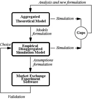
Experimental method in economics is often presented as a complementary method for the econometric one. We don’t use econometric one here, but we try1

to combine three complementary analysis levels - see Fig.#1. At the first level we found an aggregated theoretical model, a disaggregated model is at second one. The third level is an experimental one (we built an exchange software)2

. Our purpose is to compare the results of a disaggregated model, which would be chosen by experiment, with the results of an aggregated one.

Fig.#1 - Theoretical, empirical, and experimental system

Because our disaggregated model is built according to an analogical pro-cess of exchange behaviors, we think that experimental methods are able to validate it3

. Experiments help us to choose the right disaggregated model among a lot of potential one. When we examine general literature about algorithms4

(simulation or optimization one), we can observe that an ana-logical process is seldom used. If we except the commercial traveller, queue or dynamic programming algorithms, the differential criteria of the

optimiza-1

- In a preliminary working paper for a macroeconomic Doctorate thesis (R.Buda, 1997), we examine the difficulties of the behavior equations and our temporary conclusion was that we have to formalize analogical equations. So, we have considered the aggregated level was not compatible with such a formalization.

2

- We have built all the system with the language Turbo-Pascal 7.0.

3

- This reflection is born during the redaction of our Doctorate thesis (the main purpose of this thesis was to build a macro-econometric modelling software for multi-dimensional models, and so to study the relationship between algorithms and real behaviors in the mar-kets). The idea was reinforced too by some teaching experiments in high school (R.Buda, 1998).

4

tion algorithms (gradients, etc.) don’t indeed describe the behavior of the economic agents.

We have applied here our method to the price mechanism. We assume a market with only one good (in the disaggregated model, but eight in the market experiment) without any production - agents are consumers, sellers, or dealers only5

. In this paper, we’ll describe the stages of the building of the system and some applications of the disaggregated model, but not experimental results yet6

. We’ll then be able to examine some theoretical problems (price mechanism, "market socialism").

1 - The Price Mechanism Theoretical Model

The new-classical model is based on the price mechanism. Under some assumptions, it describes pure and perfect competition. Here, we tried to build an algorithm to resolve an exchange problem and then, we tried to compare its results with the theoretical equilibrium results (in the case of a partial equilibrium).

Tab#1 - Total number list of buyers and sellers for each price

Total number Total number Total number Price of potential of potential

purchases sales

P0 A0 V0

P1 A1 V1

P2 A2 V2

..

. ... ...

Pn An Vn

1.1 - Theory and Price Mecanism

The assumption we particularly examine, is the transparency one. Con-sumers and sellers are supposed rational. That means each consumer and

5

- We’ll have to leave this assumption, and we’ll have to resolve a programming difficult ; with this assumption we are not able to consider the substitutions effect between goods.

6

seller (resp.) knows his maximum purchase price and minimum sale price (resp.) - we speak about "psychological price" in commercial management. They have access neither concerning difficulties nor costs, to the information necessary for their transactions. According to static analysis7

, we assume that an auctioneer announces some prices until the number of demanders is equal to the suppliers on - "equilibrium". We often read in literature, that at each price some of them make a contract, but in the same time some others break their previous contract. Such a contract process is not right from a legal point of view8

. Well, in the experimental method we consider the role of institutions. The behavior of auctioneer is one of "tâtonnement", that means he increases or decreases (resp.) the prices when he observes an excess of demand or supply (resp.). We assume we can obtain the level of each side of the market (Demand and Supply) by aggregation (with a simple addition). In fact, such an assumption implies that each agent is able to meet all the others.

1.2 - Price Mechanism and Algorithm

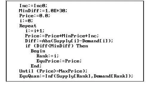
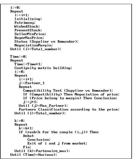
According to the new-classical model, we have built a first algorithm to calculate the equilibrium point of a market with one good. Our algorithm is simulating a kind of auction.

Fig.#2 - Price mechanism algorithm

We don’t keep the behavior pattern which we described at § 1.1 (increase and decrease movements with which auctioneer obtains equilibrium). We consider the auctioneer regularly increases ("english auction") prices from a

7

- We don’t speak about dynamic analysis (i.e. Cobweb algorithm), even if we can explain some cyclical phenomenon.

8

"bottom price". At each price, algorithm compares the number of deman-ders to the number of suppliers. In fact, we are not always able to reach perfect equilibrium (equality of the both sides total numbers). Hence, our algorithm considers that equilibrium is the point where the market minimizes the difference between both numbers - see Fig.#29

.

In fact, the market holds intrinsic social information - see Tab.#1. The new-classical model of pure and perfect competition asserts that this infor-mation is revealed by an auctioneer process (auctioneer, advertising, etc.), so that no transaction can take place outside the equilibrium. We know, with the result of experimental economics, there are a lot of transactions outside equilibrium point without any auctioneer process. Moreover, there are two grounds on which to consider a disaggregated scale of analysis. First, the conditions of validity of the Brower theorem (the continuity of the functions) are not filled - there is not always a price between two successive prices. Sec-ondly, the Sonnenschein’s theorem about the aggregation restriction10

lead us to examine the market mechanism before any data aggregation.

2 - An Empirical Disaggregated Model - SINGUL

SINGUL is a imperfect competition market (without any auctioneer pro-cess) price and quantity calculation model. Its algorithm is analogical be-cause it is built from the most realistic (as possible) behavior of the agents of a market. Our model simulates the meeting between the agents. Each agent is able to meet a limited number of other agents11

, and doesn’t know the whole information about his market12

. He is able, in a price interval, to negociate prices to make them increase or decrease (resp.) if he sells or buys (resp.) the good.

9

- Where Inc0=Price Increment between MinPrice and MaxPrice. Diff=Absolute dif-ference between Supply and Demand at the ith rank. We keep temporary the price in EquPrice (Equilibrium Price) if Diff is less than MinDiff. As soon as we reach Max-Price, the equilibrium quantity (EquQuan) become equal to the smallest value between Supply(rank) and Demand(rank).

10

- H.Sonnenschein, "Do Walras Identity and Continuity Characterize the Class of Com-munity Excess Demand ?",Journal of Economic Theory, N˚6, 1973.

11

- Even if agent uses new communication tools, this number of contacts is not propor-tional to the size of the market - see M.Polanyi (1951, in french edition 1989, pp.148–77). The limitation is not a technical one but a physiological one.

12

2.1 - Description of the Basic Model

SINGUL is a very short period model with only one good. The agents can’t stock quantity of this good over the level they indeed need. So, they can’t speculate. SINGUL simulates the behavior of the N total number of agents. For each agent SINGUL calculates13

the initial patrimony (1), initial present stock (2), wished stock14

(3), "mind price"15

- it’s a kind of hidden price : if the agent wants to buy the good, he won’t pay more than a maximum price ; if the agent wants to sell the good, he won’t to be paid less than a minimum price - (4) and (5), and the negociation margin which determines the interval of transaction.

P atrimt_i=P atrim0

i (1)

Stock_Courantt_i =Stock_Courant0

i (2)

Stock_Desiret_i =Stock_Desire0

i (3)

P rix_M axi=P rix_M axi (4)

P rix_M ini=P rix_M ini (5)

M argei=M argei (6)

The i-th agent meets a total number of Pi other agents. Their ranks are

selected by random choice among N ₋1 ranks. The i-th agent negociates

the price of one unit of the good. At the begining of the simulation, if the difference ∆t

i =Stock_Courant t

i −Stock_Desire

t

i is negative, positive

(resp.) then the agent is seller, buyer (resp.). When the difference becomes equal to zero, then the agent leaves the market.

During the negociation (9,10) between the two agentsi-th and j-th, they

won’t be motivated with the same strength. One of the both agents, who has got the greater difference (∆t

), will accept the price condition of the other agent more easily. But the conclusion of transaction happens only if the price belongs to both negociation intervals (12 to 17). Neither agent knows the negociation margin of his partner.

∆t

i=Stock_Courantti−Stock_Desireti (7)

∆t

j=Stock_Couranttj−Stock_Desiretj (8)

αt_i,j= |∆

t j|

|∆t

i|+|∆tj|

(9)

13

- We use sometimes pseudo-random procedures.

14

- It’s a kind of cardinal utility index. For J.C.HARSANYI (1956), cardinal utilities are better than ordinal one, in the bargaining mechanism analysis.

15

if

P rix_M axAcheteur< P rix_M inV endeur

then

P rixt_i,j=αt_i,j.P rixt_i+ (1−α_i,jt ).P rixt_j (10) else

P rixt_i,j=ψ.P rixt_i+ (1−ψ).P rixt_j (11)

ψ= 0

or

ψ= 1

P rixti.(1−M argei) ≤ P rixi,j (12)

P rixt_j.(1−M argej) ≥ P rixi,j (13)

∆i <0 (ibuyer) and∆j >0(jseller)

P rixt_i = P rix_M axi (14)

P rixt_j = P rix_M inj (15)

∆i >0 (iseller) and∆j <0 (jbuyer)

P rixt_i = P rix_M ini (16)

P rixt

j = P rix_M axj (17)

We have considered too that, sometimes the price order was not a normal order - i.e. the minimum price of the seller is less than the maximum price of the buyer. In this case, we assumed that only one of the two agents (he is randomly chosen) understands that the price order is abnormal. So he agrees with the price condition of the other, because it’s more interesting for him than his own. This case could lead us to examine later the negociation under the ultimatum game point of view16

.

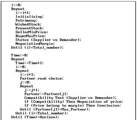
Thus, in the basic model, the agents try to reach a "level aim", (increase or decrease their good stock level) under constraints (BuyerMaxPrice, Seller-MinPrice and NegociationMargin)17

. During a simulation session, we assume

16

- There is a relationship between negociation and discrete representation of agent in an economy - see J.Neumann (Von), O.Morgenstern, The Theory of Games and Economic Behavior, New Jersey, Princeton UP, 1944. About experimental games and ultimata, see J.Ochs et A.Roth (1989).

17

- We have replace the program M axU under income constraints with the program

M in|Sc−Sd| under income constraints -Sc andSd (resp.) for present stock and wished

one agent can meet enough other agents to reach his aim and to leave the market - see algorithm in Fig.#3.

Fig.#3 - Random transactions calculation algorithm

2.2 - Some Variants of the Basic Model

If we leave the level aim assumption, we can admit that the i-th agent tries to choose the best partner (the cheapest seller or the most generous buyer) among all of the Pi agents he has met. The agents try to reach a

"price aim". In such a case, we need more periods of simulation than in the first one.

During simulation,i-th agent meets Pi partners (their rank is selected by

random choice) and he makes a classification from the best to the worse18

. If the j-th agent is selected byi-th, the transaction will be concluded only if in

the mind of thej-th agent, thei-th agent is his best partner too19

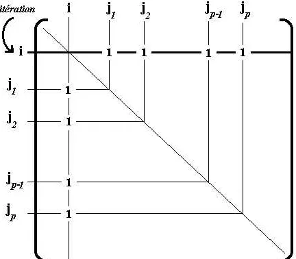
. We have to consider a symmetric relationship (i, j) and (j, i) to avoid being paradoxical : with a total random procedure we would obtain that iwould meet j but j

wasn’t met by i. So we have used a contiguity matrix20

- see Fig.#4. That

18

- In Production of Commodities by Means of Commodities (Cambridge UP, 1960), P.Sraffa assumed through a new-ricardian analysis, that consumers make classification of the sellers.

19

- The have to simulate a symmetric relationship We have used a contiguity matrix to record the relationship(i, j)and(j, i)to organize comparisons on the both sides.

20

matrix is used to keep classification too. So prices are reservation prices ; they become real prices if the couple (i, j) is optimal for both sides. Then both agents leave the market temporarily during the other negociations.

Fig.#4 - Contiguity and transactions matrix structure21

The exchange system is solved at the first level, when all the couples of agents i and j, who have drawn up contract are so that i has chosen j at first and j has chosen i at first. We write the couple is a (1,1) one. But we can solve the exchange system on a second level too. That means that we keep first all the couples (1,1), and then all the couples (1,2) & (2,1). We solve the exchange system on a third level, when we keep the (1,1), then (1,2) & (2,1), and at last the (1,3), (3,1), (3,2), (2,3), (3,3) couples. We can solve the system until the Pith level, but the agents who drawn up contracts at such a level are less useful than those who have found partners at the first level22

.

The following equations of the model are :

P rixt_i,j = h

=1

inf

Pi−r

(P rixt_j,h) (18)

P rixt_j,i = k

=1

sup

Pj−r′

(P rixt_i,k) (19)

21

- As we select the rank of thePi partenaires of thei-th agent, we put the number 1

at the row of the partner ati-th line and, in the same time, we put the number 1 at the

i-th row at the partner line. We put the number 0 elsewhere.

22

r = Rang(j)

∈ Ci (20)

r′ = Rang(i)

∈ Cj (21)

where the i-th price (a reservation price) is the best that the Pi partners

have proposed to him at level r (r′ for seller) - _i and _j belong to a _{(r, r}′₎

couple. However, after one period, some agents don’t find a partner because of their best price aim. So, we have assumed that they make their transaction conditions weak. We examine two cases : 1˚ - they make their negociation margin weak ; 2˚ - they increase their partners number (Pi), it means they

buy information - see the algorithm at Fig.#5.

Chart#1 - Satisfaction interval during price negociation23

To analyze the results at the end of simulation, we have tried to define a welfare index for each agent. If an agent has found a partner, we have considered that he could reach two extreme kinds of situation. We can admit the following convention. If the transaction price P∗ _{is just at the border of}

his negociation margin price -ma ormv (resp.) if he is buyer or seller (resp)

-, then his satisfaction is minimal. IfP∗ is just equal to his own mind price

-BuyerMaxPrice or SellerMinPrice (resp.) if he is buyer or seller (resp) - then his satisfaction is maximal24

.

23

- This Chart is analogous to the chart of utilities in the bargaining analysis. We can observe that this analysis was more interesting by utilities than the price movements through the bargaining mechanism - see e.g. A.Coddington (1968).

24

when i is buyer

Si= 1−

_{P rix}t

i,j−P0

P100−P0

(22)

with

(

P100=P rix_M axi

P0=P rix_M axi.(1 +M argei)

(23)

when i is seller

Si=

_{P rix}t

i,j−P0

P100−P0

(24)

with

(

P100=P rix_M ini

P0=P rix_M in_i.(1−M arge_i)

(25)

with i= 1 toN and j = 1 toPi.

We have defined the Satisfaction index25

Sa orSv (resp.) of the buyer or

the seller (resp.) as the difference betweenP_∗ and mind price divided by the

difference between mind price increased or decreased (resp.) with negociation margin - see Chart#1 and equations (22 to 24).

Fig.#5 - Best price transactions calculation algorithm

25

In Appendix 6.3 we can find the cohesion tests about the behavior simu-lation. The next part describes the method we’ll want to use to validate the SINGUL model. The solution of the SINGUL model is not an aggregated one, so we have to use a disaggregated tool - the experimental one.

In fact, we consider, the theoretical modelling tries to get endogenous most variables of a phenomenon, and on the contrary, experimental method tries to get them exogenous (it’s even an interactive exogenezsation one).

3 - Market Experiments with the "ÉCHANGE" Software

Market experiment - as false or real situations where some agents are playing goods supplier and demander games has existed for a long time -let’s think about the financial markets, the fish market auctions, etc. The ECHANGE software we’ll present now, explores the imperfect competition problem26

.

3.1 - The Experimental Way in Economics

The experimental method is born because on the one hand, economists attempted to abandon perfect assumptions of competition market, and on the other hand, the game theory was applied to economics and manage-ment27

. We can observe that experimental method has taken place in the teaching context too28

- or firms game context29

. The background game is often a microeconomic one, but we can imagine a macroeconomic one too30

. With such software, the pedagogical advantage is to show the mechanism of economic models to the pupils, and the experimental advantage is to collect data about economic policy decisions31

(R.Buda, 1998).

26

- One of the main problem already examined by the experiment pioneer : E.H.CHAMBERLIN, in "An Experimental Imperfect Market",Journal of Political Econ-omy, 56, 1948, pp.95–108.

27

- O.Morgenstern examined the problem of the experiment in economics - see A.Schotter (Ed.) (1976).

28

- TheJournal of Economic Education has published some experimental teaching pa-pers : R.B.Williams, Y.De Young & J.M.Leuthold in 1993 ; N.Netusil & M.J.Haupert in 1995 ; M.J.Haupert in 1996. See in French literature F.Gagey & P.Rey (1986).

29

- MIT has developed some management simulation softwares - see e.g. A.E.Amstutz (1967).

30

- By e.g., in the French literature see M.Pariset & J.M.Albertini, (Jeux et initiation économique, Paris, CNRS, 1980) or M.Berthot & S.Guillaumont-Jeanneney (Trois jeux informatiques de politique économique, Paris, Cujas, 1977) ; in the English literature see M.Binks & A.Jennings (Macroeconomics in focus, London, McGrawHill, 1986) who exam-ines rational expectations.

31

The experimental data32

has got interesting characteristics to lead a " ce-teris paribus" analysis, but we have to make some corrections33

before any interpretation. It does exist an analogy but no identity between reality and experiment. It becomes possible to lead a double complementary method (econometric and experimental one)34

. However, in our system (see Fig.#1), there is no econometric procedure. The experimental software organizes ex-changes and collects data to help disaggregated model choice.

According to V.L.Smith (1989), the choice of environment and institu-tions by the economists is the main advantage of experiment in comparison to the econometrics method. The experimental protocol is defined by five prin-ciples : 1˚- insatiability - the utility function of each agent is a monotonous function of his gains ; 2˚ - prominence - the gains of each agent depend on the actions of the other ; 3˚ - dominance - the reward motivates each agent ; 4˚ secret each agent only knows his owns information ; 5˚ parallelism -laboratory institution has to look like the real world we try to represent.

3.2 - Description of an Experimental Economics Software - "ECHANGE"

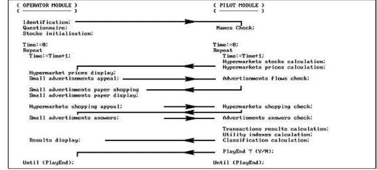
ECHANGE software can (will be able to) run under two modes on a network system. The teacher e.g., can lead the system with the pilot mode and his pupils (or students) use operator mode - see Fig.#6 - but the pilot is not an auctioneer.

Fig.#6 - ECHANGE software algorithms

32

- The data we obtain in situ are called field-happenstance-data ; the other are the laboratory-happenstance-data.

33

- It exists some econometric procedures to obtain better data (R.Deloche, 1995).

34

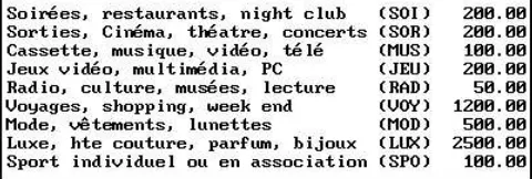
ECHANGE software simulates the transactions : the operator nor really buys the goods neither do these goods really exist. The exchanges take place over a short period (we assume a daily period) and the goods have been chosen among the leisure of the pupils - parallelism principle - see Fig.#7. Each operator exists for the other one through his advertisement(s). At each period, the operator can write advertisements and/or answer to one (to buy and/or sell), and/or buy goods at hypermarkets. They have to pay for infor-mation (advertisements, hypermarket prices) - principle of secret. We have used the hypermarkets to give a reference price of the goods - parallelism principle. At each period, ECHANGE simulates hypermarkets out of stock, very early - we want to avoid operators only buying at hypermarkets - prin-ciple of parallelism too. The goal of each operator (pupils) is to maximize his utility (in buying or selling some goods) with his liquid assets. Before the exchanges, each operator answers to a questionnaire to define his util-ity function (proportions of goods to hold at each period). Initial dotations of goods are calculated to present an excess quantity of one good, so that all operators would be sellers of one good, at least. There is no point in the operators speculating because they don’t realize their periodical aim -prominence principle. ECHANGE software calculates the classification of the operators at each period - insatiability and dominance principles -, and at the end of game - it considers the final level of liquid assets too.

3.3 - The Perspectives with "ECHANGE" software

4 - Market, Planning, and Calculation: a Temporary Conclusion

When we are writing this paper, the experiment is not applied to choose a good version of the disaggregated model SINGUL. We are not able to con-clude either the comparison or about the experiment but we hope from it, to know more about information search behaviors and the market coordination assumption. We know the transparency assumption is a controversial point. For new-keynesians R.W.Clower & A.Leijonhufvud35

, the agents make non optimal decisions because of a lack of information. For F.A.Hayek on the contrary, there is a coordination between agents in the market because no-body knows the "whole information" ; so agents look for a partner who is able to give him complementary information36

. However, we can present some reflections about the building of economic algorithms (especially ana-logical ones) and their properties in representing economic reality. When we have to build a disaggregated model, there are new problems we don’t have to resolve in comparison to aggregated ones37

. The exactness of the method depends on the solution of such a problem38

.

Our system only presents exchange models (without production), but we can reconsider here the Mises-Hayek-Lange debate39

. With all necessary in-formation and a very efficient computer, is a Planning administrator able to take place of each agent to calculate their optimal decisions - L.Mises explains us it’s impossible and for F.A.Hayek, he is necessarily inefficient ? So O.R.Lange proposed decentralizing planning40

which controled only

in-35

- "The Coordination of Economic Activities", American Economic Review, Vol.65, 1975, pp.182–88.

36

- The coordination assumption is a controversial point even in Austrian economics school - see M. Rothbard,The Ethics of Liberty, Humanities Press, Atlantic Highlands, 1982.

37

- At the level of an aggregated firm we don’t have to check all the relationships between all agents to be sure the system is coherent. We assume the necessarily relationship exist. At the disaggregated level we have to check all the relationships. In national account first, we work with aggregated data and we use some black boxes (by e.g. the "comptes écrans") to simulate the market relationship. Secondly, the national account has not gor the same properties like double-entry firms accounts - see O.Arkhipoff, "Importance et diversité des problèmes d’agrégation en Comptabilité nationale", in E.Archambault & O.Arkhipoff (EDS),La comptabilité nationale face au défi international, Paris, Economica, 1990, pp.365–81.

38

- See the macro-account building of M.Allais (1954).

39

- See L.Mises (Von) (1935), F.A.Hayek (Von)(Ed.) (1935), O.R.Lange (1967) and "On the Economic Theory of Socialism",Review of Economic Studies, N˚4(1–2), 1936-37, Reprint 1967.

40

termediate goods but the real problems of planning were never resolved41

. Because, without any prices, these economies can’t find their optimal situa-tion, moreover, the agent keeps the information (F.A.Hayek (Ed.) (op.cit.)) to keep their power - even with decentralized planning. In fact, sometimes, when one agent has to make a decision, his behavior depends on his envi-ronment. If something was different in his environment, perhaps he have made another decision. The fundamental problem is if we want to replace agent’s behavior (with planning), we try to replace some contingent actions by a few necessary procedures. For E.Barone (1908), it’s useless to calculate the exchange solution that we can obtain easily by the market mechanism without any calculation. Another point we can examine when we build algo-rithms is the arithmetical one42

. Let’s assume a planning administrator who has access to all necessary information - it would be not enough even if the agent gave their mind prices43

. Let’s assume - with the SINGUL model - that the population of an economy is 1,000,000, the number of different goods is 1,000, then the number of negociations would be 1013 (with 100 meetings for each agent), and 1021 (if each agent meets the other). Two problems occur : 1˚- the calculation duration is one month (with a 1 GHz processor) ; 2˚- the overflow of the twenty digits computers so we loose the accuracy of the calcu-lation44

. We know that it’s possible to correct the accuracy problem, but we use more calculation time. Moreover, it is not necessarily more interesting to organize a general meeting (each agent meets the other), because in this case the number of meetings will reinforce the bad position of the less interesting agents toward his partners (they can better make comparisons). When we’ll collect and we’ll analyze data and then results, we’ll have to remember these last reflections. A quantitative tool, especially a scientific one, is useful as soon as we know its limits.

too. About decentralizing planning algorithms, see P.Picard,Procédures et modèles de la planification décentralisée, Paris, Economica, 1979.

41

- Programming technicals have make progress with the work of L.V. Kantorovitch, but not the socialist planning.

42

- O.Morgenstern (1950) speaks about calculate accuracy, the heavy quantity of equa-tions to formalize and to resolve exchanges just for a very little economy. L.Robbins (The Great Depression, London, Macmillan, 1934) speak about one million equations, F.A.Hayek (Ed.)(1935, op.cit.) about a hundred millions.

43

- See the conclusion of X.Freitas (1978).

44

References

Allais M., (1954), Les fondements comptables de la macroéconomique, PUF, 96 p., (Réimpr.1993)

Amstutz A.E., (1967), Computer Simulation of Competitive Market Re-sponse, Cambridge, MIT Press, 457 p.

Barone E., (1908), "The Ministry of Production in the Collectivist State", in F.A.Hayek (Von)(Ed.), Collectivist Economic Planning, London, Rout-ledge & Sons, pp.245–90, (Reprint 1935).

Buda R., (1996), "Présentation d’un outil de contrôle de la précision des calculs en modélisation macroéconomique", Mimeo GAMA, University of Paris X-Nanterre, august.

Buda R., (1997), "La modélisation macroéconomique comme processus de communication : réflexions pour une formalisation finaliste des équations de comportement", Mimeo GAMA, University of Paris X-Nanterre, may.

Buda R., (1998), "La simulation économique : expérimentation et ap-prentissage de la réalité économique", Revue internationale de systémique, 12(2), pp.203–24.

Coddington A., (1968),Theories of Bargaining Process, London, G.Allen, 106 p.

Courbis R., (1977), Modèles de prix pour la prévision et la planification, Paris, Dunod, 435 p.

Deloche R. (1995), "Expérimentation, science économique et théorie des jeux - nunc est bibendum",Revue économique, 46(3), pp.951–60.

De Young Y., (1993), "Market Experiment : The Laboratory versus the Classroom", Journal of Economic Education, 24(4), pp.335–51.

Freitas X., (1978), Planification en environnement aléatoire - essai sur le rôle de l’information dans les procédures de planification, Doctorate Thesis, University of Toulouse, 461 p.

Gagey F. & P.Rey, (1986), "L’économie expérimentale comme outil péd-agogique - élaboration d’un jeu d’initiation à la micro-économie", Revue économique, 37(1), pp.5–30.

Harsanyi J.C., (1956), "Approaches to the Bargaining Problem before and after the Theory of Games : A Critical Discussion of Zeuthen’s, Hick’s and Nash’s Theories", Econometrica, 24, pp.144–57.

Haupert M.J., (1996), "Labor Market Experiment",Journal of Economic Education, 27(4), pp.300–08.

Hayek F.A. (Von) (Ed.), (1935),Collectivist Economic Planning, London, Routledge & Sons, 293 p.

Lalonde R.J., (1986), "Evaluating the Econometric Evaluations of Train-ing Programs with Experimental Data",American Economic Review, 76(4), pp.604–20.

Lange O.R., (1967), "The Computer and the Market", in C.H.Feinstein (Ed.), Socialism, Capitalism and Economic Growth, Cambridge, Cambridge UP, pp.158–61.

Lange O.R., (1970), Introduction to economic cybernetics, Pergamon Press, Oxford, 183 p.

Leuthold J.M., (1993), "A Free-Rider Experiment for the Large Class",

Journal of Economic Education, 24(4), pp.353–63.

Ochs J. & A.Roth, (1989), "An Experimental Study of Sequential Bar-gaining", American Economic Review, 79(3).

Marchal J., (1969), Le mécanisme des prix, Paris, M.T.Génin, 460 p. Mises L.(Von), (1935), "Les équations de l’économie mathématique et le problème du calcul économique en régime socialiste", Revue d’économie politique, 97(6), pp.899–906, (Reprint 1987).

Morgenstern O., (1950), On The Accuracy of Economic Observations, New York, Princeton UP.

Morgenstern O., (1976), "Experiment and Large Scale Computation in Economics", in A.Schotter (Ed.),Selected Economic Writings of Oskar Mor-genstern, New York, New York UP, pp.405–38.

Netusil N.R. & M.J.Haupert, (1995), "The Economics of Information - A Classroom Experiment",Journal of Economic Education, 26(4), pp.357–63. Polanyi M., (1951), The Logic of Liberty - Reflections and Rejoinders, Chicago, University of Chicago Press.

Scarf H., (1967), "On the Computation Equilibrium Prices", in W. Fellner et al. (Eds), Ten Economic Studies in the Tradition of Irving Fisher, New York, J.Wiley & Sons, pp.207–30.

Smith V.L., (1989), "Theory, Experiment and Economics", Journal of Economic Perspectives, 3, pp.151–69.

6 - Appendix

6.1 - Check Screen of the Program "ECHANGE"

Screen#1

Screen#2

Screen#3

Screen#4

Screen#5

Screen #1 gather data about pat-rimonies (current inventories, liquidi-ties) and goals (wished inventories).

Screen #2 gets information’s pur-chase tariffs.

Screen #3 provides the hypermar-ket’s merchandizes prices.

Screen #4 waits for the announce-ments.

6.2 - Description of the Market Simulation with the "ECHANGE" software

Game session stages :

At the beginning, we ask his name and its leisures preference to each operator (we try to install in a few different rooms to avoid any trouble communications). We can then calculate good stock aim utility function and initial present stocks - see Appendix 6.1.

#1 - The some information prices (Hypermarkets advertising, transport, advertisement) are displayed (local one are free).

#2 - Operator can "write" advertisement (to buy vs sale purchases). He can keep one message during a lot of period. Price is lower than normal message, but he can’t change the message until of the total of period.

#3 - Operator can buy the advertisements national paper (local one is free). After the second display of advertisements, operator has to pay.

#4 - Operator can answer to one or a lot of advertisements. Who answer do accept to pay for transport of good. When he answer, transaction is not warranted. Perhaps there are a lot of answers to the same advertise-ment. The first arrived is the partner.

#5 - Operator can buy the same kind of goods in hypermarkets.

#6 - Software calculates transaction results. Then results are displayed at each screen. Utility functions and new classification are calculated and possibly displayed. Some parameters in the utility are implemented to avoid the explosive classification (one operator is first and the other know they never reach him).

In the goods file we can find the name of each one, and the reference hypermarket price - see Fig.#7.

R odol phe B u da, G A M A -M O D E M C N R S , U n iv er si ty of P ar is 10

MARCHE DE 20 OPERATEURS

10 VENDEURS ET 10 ACHETEURS ETAT DES PATRIMOINES

1 ACH -2 57.6000 16.3000 0.350 19200.0000 5 -2 ACH -3 39.5000 19.5000 0.390 17500.0000 5 -3 VEN 2 54.5000 20.0000 0.310 17800.0000 5 -4 ACH -4 40.0000 21.7000 0.360 19200.0000 5 -5 VEN 2 41.3000 37.0000 0.320 16900.0000 5 -6 VEN 1 50.0000 34.7000 0.310 18500.0000 5 -7 VEN 1 49.3000 20.4000 0.350 17200.0000 5 -8 ACH -2 41.3000 16.3000 0.380 19400.0000 5 -9 VEN 1 53.0000 23.4000 0.350 19900.0000 5 -10 VEN 4 48.9000 36.2000 0.390 16600.0000 5 -11 VEN 2 54.7000 38.5000 0.340 16500.0000 5 -12 ACH -1 38.4000 35.5000 0.350 18500.0000 5 -13 VEN 3 45.9000 26.8000 0.320 18800.0000 5 -14 ACH -4 54.7000 27.0000 0.370 17300.0000 5 -15 ACH -2 48.9000 15.2000 0.370 18900.0000 5 -16 VEN 3 51.8000 36.5000 0.340 17900.0000 5 -17 ACH -2 36.0000 21.9000 0.310 19000.0000 5 -18 ACH -2 59.2000 20.9000 0.310 17200.0000 5 -19 VEN 2 46.3000 39.7000 0.350 18000.0000 5 -20 ACH -1 47.4000 22.1000 0.400 17000.0000 5 -DELTA STOCKS 21 -23

PERIODE 1

PRIX D’EQUILIBRE 38.3740 QUTE D’EQUILIBRE 0 RESOLUTION DU MARCHE ETAPE 1 --- ( 5/ 14) 36.5333 ( 13/ 12) 38.1000

FIN DES TRANSACTIONS ---NOMBRE DE TRANSACTIONS 2 POURCENTAGE DE TRANSACTION 20.0000%

PRIX MOYEN DE TRANSACTION 37.3167 PRIX MODAL DE TRANSACTION 36.5000 DELTA STOCKS 2 -5

ETAT DES PATRIMOINES

1 ACH -2 16.3000 0.350 19200.0000 5 -2 ACH -3 19.5000 0.390 17500.0000 5 -3 VEN 2 54.5000 0.310 17800.0000 5 -4 ACH -4 21.7000 0.360 19200.0000 5 -5 VEN 1 41.3000 0.320 16936.5333 5 0.639 6 VEN 1 50.0000 0.310 18500.0000 5

-7 VEN 1 49.3000 0.350 17200.0000 5 -8 ACH -2 16.3000 0.380 19400.0000 5 -9 VEN 1 53.0000 0.350 19900.0000 5 -10 VEN 4 48.9000 0.390 16600.0000 5 -11 VEN 2 54.7000 0.340 16500.0000 5 -12

13 VEN 2 45.9000 0.320 18838.1000 5 0.469 14 ACH -3 27.0000 0.370 17263.4667 5 0.954 15 ACH -2 15.2000 0.370 18900.0000 5 -16 VEN 3 51.8000 0.340 17900.0000 5 -17 ACH -2 21.9000 0.310 19000.0000 5 -18 ACH -2 20.9000 0.310 17200.0000 5 -19 VEN 2 46.3000 0.350 18000.0000 5 -20 ACH -1 22.1000 0.400 17000.0000 5 -DELTA STOCKS 19 -21

PERIODE 2

PRIX D’EQUILIBRE 34.1240 QUTE D’EQUILIBRE 0 RESOLUTION DU MARCHE ETAPE 1 --- ( 19/ 20) 30.1667

FIN DES TRANSACTIONS ---NOMBRE DE TRANSACTIONS 1 POURCENTAGE DE TRANSACTION 10.0000%

PRIX MOYEN DE TRANSACTION 30.1667 PRIX MODAL DE TRANSACTION 30.2500 DELTA STOCKS 2 -5

ETAT DES PATRIMOINES

1 ACH -2 16.3000 0.350 19200.0000 5 -2 ACH -3 19.5000 0.390 17500.0000 5 -3 VEN 2 54.5000 0.310 17800.0000 5 -4 ACH -4 21.7000 0.360 19200.0000 5 -5 VEN 1 41.3000 0.320 16936.5333 5 0.639 6 VEN 1 50.0000 0.310 18500.0000 5 -7 VEN 1 49.3000 0.350 17200.0000 5 -8 ACH -2 16.3000 0.380 19400.0000 5 -9 VEN 1 53.0000 0.350 19900.0000 5 -10 VEN 4 48.9000 0.390 16600.0000 5 -11 VEN 2 54.7000 0.340 16500.0000 5 -12

-E x chan ge M ode lli n g E x pe ri m en t, S im u lat ion A lg or it hm s, an d T he or et ic al A n al y si s 23

DELTA STOCKS 18 -20 PERIODE 3

PRIX D’EQUILIBRE 34.1240 QUTE D’EQUILIBRE 0 RESOLUTION DU MARCHE ETAPE 1 --- ( 10/ 14) 36.3857

FIN DES TRANSACTIONS ---NOMBRE DE TRANSACTIONS 1 POURCENTAGE DE TRANSACTION 10.0000%

PRIX MOYEN DE TRANSACTION 36.3857 PRIX MODAL DE TRANSACTION 36.5000 DELTA STOCKS 2 -5

ETAT DES PATRIMOINES

1 ACH -2 16.3000 0.350 19200.0000 5 -2 ACH -3 19.5000 0.390 17500.0000 5 -3 VEN 2 54.5000 0.310 17800.0000 5 -4 ACH -4 21.7000 0.360 19200.0000 5 -5 VEN 1 41.3000 0.320 16936.5333 5 0.639 6 VEN 1 50.0000 0.310 18500.0000 5 -7 VEN 1 49.3000 0.350 17200.0000 5 -8 ACH -2 16.3000 0.380 19400.0000 5 -9 VEN 1 53.0000 0.350 19900.0000 5 -10 VEN 3 48.9000 0.390 16636.3857 5 0.344 11 VEN 2 54.7000 0.340 16500.0000 5 -12

13 VEN 2 45.9000 0.320 18838.1000 5 0.469 14 ACH -2 27.0000 0.370 17227.0810 5 0.940 15 ACH -2 15.2000 0.370 18900.0000 5 -16 VEN 3 51.8000 0.340 17900.0000 5 -17 ACH -2 21.9000 0.310 19000.0000 5 -18 ACH -2 20.9000 0.310 17200.0000 5 -19 VEN 1 46.3000 0.350 18030.1667 5 0.004 20

DELTA STOCKS 17 -19 PERIODE 4

PRIX D’EQUILIBRE 34.1240 QUTE D’EQUILIBRE 0 RESOLUTION DU MARCHE ETAPE 1 --- ( 5/ 14) 36.5333

FIN DES TRANSACTIONS ---NOMBRE DE TRANSACTIONS 1

ETAT DES PATRIMOINES

1 ACH -2 16.3000 0.350 19200.0000 5 -2 ACH -3 19.5000 0.390 17500.0000 5 -3 VEN 2 54.5000 0.310 17800.0000 5 -4 ACH -4 21.7000 0.360 19200.0000 5 -5

6 VEN 1 50.0000 0.310 18500.0000 5 -7 VEN 1 49.3000 0.350 17200.0000 5 -8 ACH -2 16.3000 0.380 19400.0000 5 -9 VEN 1 53.0000 0.350 19900.0000 5 -10 VEN 3 48.9000 0.390 16636.3857 5 0.344 11 VEN 2 54.7000 0.340 16500.0000 5 -12

13 VEN 2 45.9000 0.320 18838.1000 5 0.469 14 ACH -1 27.0000 0.370 17190.5476 5 0.954 15 ACH -2 15.2000 0.370 18900.0000 5 -16 VEN 3 51.8000 0.340 17900.0000 5 -17 ACH -2 21.9000 0.310 19000.0000 5 -18 ACH -2 20.9000 0.310 17200.0000 5 -19 VEN 1 46.3000 0.350 18030.1667 5 0.004 20

DELTA STOCKS 16 -18 PERIODE 5

PRIX D’EQUILIBRE 36.4240 QUTE D’EQUILIBRE 0 RESOLUTION DU MARCHE ETAPE 1 --- ( 10/ 14) 32.4750

FIN DES TRANSACTIONS ---NOMBRE DE TRANSACTIONS 1 POURCENTAGE DE TRANSACTION 10.0000%

PRIX MOYEN DE TRANSACTION 32.4750 PRIX MODAL DE TRANSACTION 32.2500 DELTA STOCKS 2 -5

ETAT DES PATRIMOINES

1 ACH -2 16.3000 0.350 19200.0000 5 -2 ACH -3 19.5000 0.390 17500.0000 5 -3 VEN 2 54.5000 0.310 17800.0000 5 -4 ACH -4 21.7000 0.360 19200.0000 5 -5

R odol phe B u da, G A M A -M O D E M C N R S , U n iv er si ty of P ar is 10 14

15 ACH -2 15.2000 0.370 18900.0000 5 -16 VEN 3 51.8000 0.340 17900.0000 5 -17 ACH -2 21.9000 0.310 19000.0000 5 -18 ACH -2 20.9000 0.310 17200.0000 5 -19 VEN 1 46.3000 0.350 18030.1667 5 0.004 20

DELTA STOCKS 15 -17 PERIODE 6

PRIX D’EQUILIBRE 33.8740 QUTE D’EQUILIBRE 0 RESOLUTION DU MARCHE

AUCUNE TRANSACTION ---ETAT DES PATRIMOINES

1 ACH -2 16.3000 0.350 19200.0000 5 -2 ACH -3 19.5000 0.390 17500.0000 5 -3 VEN 2 54.5000 0.310 17800.0000 5 -4 ACH -4 21.7000 0.360 19200.0000 5 -5

6 VEN 1 50.0000 0.310 18500.0000 5 -7 VEN 1 49.3000 0.350 17200.0000 5 -8 ACH -2 16.3000 0.380 19400.0000 5 -9 VEN 1 53.0000 0.350 19900.0000 5 -10 VEN 2 48.9000 0.390 16668.8607 5 0.139 11 VEN 2 54.7000 0.340 16500.0000 5 -12

13 VEN 2 45.9000 0.320 18838.1000 5 0.469 14

15 ACH -2 15.2000 0.370 18900.0000 5 -16 VEN 3 51.8000 0.340 17900.0000 5 -17 ACH -2 21.9000 0.310 19000.0000 5 -18 ACH -2 20.9000 0.310 17200.0000 5 -19 VEN 1 46.3000 0.350 18030.1667 5 0.004

ETAT DES PATRIMOINES

1 ACH -2 57.6000 16.3000 0.350 19200.0000 5 -2 ACH -3 39.5000 19.5000 0.390 17500.0000 5 -3 VEN 2 54.5000 20.0000 0.310 17800.0000 5 -4 ACH -4 40.0000 21.7000 0.360 19200.0000 5 -5 XXX 0 41.3000 37.0000 0.320 16973.0667 5 0.639 6 VEN 1 50.0000 34.7000 0.310 18500.0000 5 -7 VEN 1 49.3000 20.4000 0.350 17200.0000 5 -8 ACH -2 41.3000 16.3000 0.380 19400.0000 5 -9 VEN 1 53.0000 23.4000 0.350 19900.0000 5 -10 VEN 2 48.9000 36.2000 0.390 16668.8607 5 0.139 11 VEN 2 54.7000 38.5000 0.340 16500.0000 5 -12 XXX 0 38.4000 35.5000 0.350 18461.9000 5 0.209 13 VEN 2 45.9000 26.8000 0.320 18838.1000 5 0.469 14 XXX 0 54.7000 27.0000 0.370 17158.0726 5 0.548 15 ACH -2 48.9000 15.2000 0.370 18900.0000 5 -16 VEN 3 51.8000 36.5000 0.340 17900.0000 5 -17 ACH -2 36.0000 21.9000 0.310 19000.0000 5 -18 ACH -2 59.2000 20.9000 0.310 17200.0000 5 -19 VEN 1 46.3000 39.7000 0.350 18030.1667 5 0.004 20 XXX 0 47.4000 22.1000 0.400 16969.8333 5 0.913 DELTA STOCKS 15 -17

SATISFACTION-PRIX MOYENNE DES ACHETEURS 0.000 SATISFACTION-PRIX MOYENNE DES VENDEURS 0.204 PRIX D’EQUILIBRE 33.8740 QUTE D’EQUILIBRE 0 MARCHANDISE EN SURPLUS 15 / 21 DEMANDE NON SATISFAITE 17 / 23

TAUX DE SATIETE DU MARCHE 20.00%