An Intelligent Model in Bioinformatics based on
Rough-Neural Computing
Ahmed Abou El-Fetouh S
.1 *iMona Gamal
2Mansoura University, Faculty of Computer and Information Sciences Information System Department
1
Head of the department , 2Assistant Lecturer
P.O.Box: 35516
ABSTRACT
The bioinformatics field is concerned with processing medical data for information and knowledge extraction. The problem comes more interesting when dealing with uncertain data which is very common in the medicine diagnostic area. The medical data is processed inside the human brain to produce the appropriate diagnoses. The artificial neural networks are simulations to the human thinking. The rough neural networks are special networks that are capable of dealing with rough boundaries of uncertainness through rough neurons. This research tries to solve the diagnostic problems using the classification capabilities of the rough neural networks. The medical training data ,after preprocessing to remove unnecessary attributes, are applied to the rough neural network structure so as to update the connection weights iteratively and produce the final network that give a good accuracy rates. The testing data are used to measure these accuracy rates. The input data are transformed into its lower and upper boundaries by multiplying them by the input weights so there are no need for preparing rough data in advance. The illustrations of the proposed model and its sub modules along with the experimental results and comparisons with the neural network in diagnosing medical knowledge from the breast cancer data set for a number of experiments with different training set sizes are declared.
General Terms
Data Mining, Bioinformatics.Keywords
Uncertain knowledge, Rough Neural Networks.
1.
INTRODUCTION
The biomedical information system [1] is concerned with structuring, storing and processing medical data for different reasons. One of these is to help doctors diagnose their patient's illness through a good and accurate decision support system DSS [2]. DSS were initially designed to help decision makers to solve badly structure or multi featured problems. Over the years DSS where motivated to be intelligent by using artificial intelligence (AI) [3] techniques in data preprocessing and decision (knowledge) extraction to help decision maker be more accurate in solving his problems. The AI techniques are different and each one has its own abilities and limitations so they are chosen according to the problems in hand.
Artificial Neural Networks (ANNs)[4] are computational tools (AI technique) which were found to be very strong in solving pattern recognition and decision support problems specially in the field of biomedical sciences after the development of the
back-propagation algorithm[5]. ANNs are simulations to human brain and its ability to think and conclude knowledge from concrete data. They are composed of layers of neurons (biological learning and memory cells) which are connected to each other using weighted connections (synapses). The ANNs do not need any rules to be figured out as they adjust their weights according to input/output data and error rate using the correct algorithm contrasting with expert system that their accuracy depends on the rules they work on and these rules are very hard to be extracted correctly. Rough Neural Networks (RNNs) [5, 6, 7, 8, and 9] are an upgrade of the ANN. RNN makes use of the rough set theory to deal with uncertainness levels. RNNs are built to care for vague boundaries of uncertainness through lower and upper neurons. The input rough neurons take the data as lower and upper bounds and process them through the network producing the corresponding output. This makes RNNs much better for medical cases which data is probabilistic and uncertain.
Many researchers have introduced RNNs in their work for classification and decision making systems. One research used RNN in image processing domain by combining rough sets and adaptive neural networks [10]. An other approach used a hybrid of rough sets and artificial neural networks for failure domain prediction in telecommunication networks [11]. An other research used BP neural network with rough set for short term load forecasting [12]. Hand-written character recognition is implemented by the data mining and knowledge discovery software system RoughNeuralLab [13]. A method to develop rough neural network of variable precision and train it using Levenberg–Marquart algorithm is presented in the RNNs applications as well[14].
with neural networks working on the same data set is declared in section 4. Finally the conclusion of the research is in section 5.
2.
Theoretical Bases
2.1 Rough Set Theory
Rough set theory has been introduced by Professor Pawlak to extract classification rules from uncertain and vague data sets [15, 16]. It is based on the concept of an upper and a lower approximation of a set. Each uncertain feature space is a disjoint of the two approximations. Rough set analysis depends on the data set without the need for any other external parameters.
An information system (IS) is an ordered pair (U, A), where U = {x1, x2 . . xn} is a nonempty finite set of objects called the
universe, and P = {p1, p2, . . . , pn}is a nonempty set and the
elements of P, called attributes ( in our case called medical features).
A rough set [17] is an approximation of an uncertain concept by a pair of precise concepts, called lower and upper approximations (which are informally a classification of the domain of interest into disjoint categories). Objects belonging to the same category characterized by the same attributes (or features) are not distinguishable.
LetXU be a target set that we wish to represent using
attribute subset
P
. The tuple(
P
X
,
P
X
)
composed of thelower and upper approximation represent the rough set. Thus, a rough set is composed of two crisp sets, one representing a lower boundary of the target set
X
, and the other representing an upper boundary of the target setX
. This means that the target setX
can be approximated using only the information contained withinP
by constructing theP
-lower andP
-upper approximations ofX
:}
]
[
|
{
x
x
p
X
X
P
(1)}
]
[
|
{
x
x
p
X
X
P
(2)2.2 Rough Neural Network
Rough neural networks[6,7,8,9,and 10] are like conventional neural networks in their training algorithms and connection mode, but they differ in the neuron used in the network . Instead of the conventional neuron the rough neural use a pair of neurons to represent the rough neuron. One for the upper approximation and the other for the lower approximation of the feature or attribute that the neuron represents. A back propagation network in the rough mode is composed of three layers. The input layer is composed of the features used in the model which the rough neural network used to simulate. Each feature is represented by two neurons connected imaginary with each other to facilitate information exchange. The input feed comes to the lower and upper neurons from the external world and first multiplied by a weight connection connected to the neurons. This weight connection is updated during the
learning phase along with other weighted connections in the network. The hidden layer is composed of a number of rough neurons calculated by the Baum-Haussler rule[18]:
o I
e ts hn
N
N
T
*
N
N
(3)Where Nhn is the number of hidden neurons, Nts is the number
of training samples,
Te is the tolerance error, NI is the number of inputs ( attributes
or features), and No is the number of the output.
Each neuron in the hidden layer is actually represented by two neurons which take its input feed from the input layer. This can be expressed as if each of the input and hidden layers contains two sub layers one for lower approximation and the other for upper approximation. The lower approximation neurons in the input layer are fully connected to the lower approximation neurons in the hidden layer and in the same way the upper approximation neurons are connected. The output layer is composed of one conventional neuron to produce the output of the network. The connections between the hidden layer and output layer is a full connection mode but the lower and upper neurons in the hidden layer are treated as if they were rough neurons producing only one output and one connection weight for each rough neuron.
The output of a rough neuron is a pair of upper and lower bounds, while the output of a conventional neuron is a single value. Let (ILn,OLn) is the input/output of the lower rough neuron and (IUn,OUn) is the input/output of the upper rough neuron. The calculation of the input/output of the lower/upper rough neuron is given by the following equations:
O wL I
n
j
nj nj
Ln
1
(4)
1
n
j
nj nj
U wU O
I n (5)
))
), f(I
Min(f(I
O
Ln
Ln Un (6)))
), f(I
Max(f(I
O
Un
Ln Un (7)Where f is the transfer function used to calculate the activation of the neurons and would be the sigmoid function.
x
e
x
f
1
1
)
(
(8)Where x is the neuron input and λ is a constant which its value is chosen according to experiments.
Ln
Un
O
O
O
(9)The previous equations are used to calculate the output from the hidden neurons layer to the output neuron . Only equations 4, 5, 6 and 7 are used to calculate the lower and upper neurons output from input layer to hidden layer.
3.
The Proposed Model
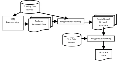
The proposed model is a transform hybrid model that is composed a preprocessing sub module and a training rough neural module. Figure 1 shows the main sub modules and their input/output structure .
The proposed model is composed of three main modules which are :
(1)Data Preprocessing : this module is responsible for managing the medical data introduced to the system for farther classification. The management includes the data reduction which is removing the unnecessary attributes that do not contribute in the classification process. (2)The Rough Neural Network Training Module :which
takes the training data set and apply them to the network structure to modify the connecting weights and produce the final network structure.
(3)The Rough Neural Network Testing Module: that applies the testing data set to the network and computes the accuracy in terms of the absolute error rate.
3.1 Medical Data Preprocessing
The data preprocessing is essential in terms of reducing time and space consumption. The medical data that is needed to be applied to the rough neural network are to be preprocessed first. This phase is implemented by the weka data miner tool. Weka supervised attribute filter can be used to select attributes. It is very flexible and allows various evaluation and search methods to be combined. The evaluator used is CfsSubsetEval[19] which determines how attributes/attribute subsets are evaluated. It evaluates the worth of a subset of attributes by considering the individual predictive ability of each feature along with the degree of redundancy between them.
The search method is the Best First algorithm[20]. It searches the space of attribute subsets by greedy hillclimbing[21] augmented with a backtracking facility. Setting the number of consecutive non-improving nodes allowed controls the level of backtracking done. Best first may start with the empty set of attributes and search forward, or start with the full set of
attributes and search backward, or start at any point and search in both directions (by considering all possible single attribute additions and deletions at a given point).
The output of that phase is the reduced data set that is ready for classification.
3.2 Rough Neural Networks For
Classifying Medical Data
This module handles the implementation of the rough neural network structure and applying the training data on the network for the learning process. The input features data will be ordinary data no rough data boundaries but the each feature input will be multiplied once by the input weight connection of the lower approximation input layer neuron and the other by the input weight connection of the upper approximation neuron. These input connections will be updated during the weight update phase to model the lower and upper boundaries of each input feature. The ordinary data can then be used directly as an input data with out the need for further processing to get the lower and upper data boundaries.
The structure of the network is illustrated in figure 2
The training of the rough back propagation neural network is just like the conventional one but the equations in section are used to calculate the output of lower and upper neurons in both the input and the hidden layer. The conventional neuron in the output layer is calculated by the transfer function. The transfer function used in this model is the sigmoid function illustrated by the equation 8:
Phase 1: Propagation
Each propagation involves the following steps:
1. Forward propagation of a training pattern's input through the rough neural network in order to generate the propagation's output activations for all lower and upper neurons and conventional neurons in the network.
2. Backward propagation of the propagation's output activations through the rough neural network using the training pattern's target in order to generate the deltas (error rate) of all output and hidden neurons.
Phase 2: Weight update
For each weight-synapse follow the following steps:
L U
L U
L U
O L
U
L U L
U Feature 1
Output Layer Input layer Hidden Layer
Feature 2
Feature n wl
wu
[image:3.595.321.551.366.494.2]wij
[image:3.595.64.269.400.508.2]Figure 2 : the Rough Neural Network Structure
Figure 1: Rough Neural Network model in classifying uncertain Data
Data
Preprocessing Reduced Featured Data
Rough Neural Training Training Data
records
Test Data records
Rough Neural Testing Rough Neural
Network Structure
1. Multiply its output delta and input activation to get the gradient of the weight.
2. Bring the weight in the opposite direction of the gradient by subtracting a ratio of it from the weight. This ratio influences the speed and quality of learning; it is called the learning rate. The sign of the gradient of a weight indicates where the error is increasing, this is why the weight must be updated in the opposite direction.
neuron)) (input activation * learnRate * Derivative * error ( ij w old ij w
new (10)
Repeat phase 1 and 2 until the performance of the network is satisfactory.
Actual algorithm for a 3-layer rough neural network (only one hidden layer):
Step1 : Initialize the weights in the network (often randomly)
Step2 : Do
Step3 : For each example t in the training set
Step4 : O = rough neural-net-output(network, t) ; forward pass //(actual output)
Step5 : T = target output for t
Step6: Calculate error (T - O) at the output units Step7: Compute delta_wh for all weights from hidden layer to output layer ; backward pass
Step8 : Compute delta_wli for all weights from input lower approximation layer to hidden lower approximation layer ; backward pass continued
Step9 : Compute delta_wui for all weights from input upper approximation layer to hidden upper approximation layer ; backward pass continued Step10 : Compute delta_wl and delta_wu for each lower and upper approximation neuron in the input layer ; backward pass continued
Step11 : Update the weights in the network
Step12 : Until all examples classified correctly or stopping criterion satisfied Return the network.
The output of that module is a good trained rough neural network structure that is capable of classifying new data records according to the inputs and connection weights (updated during the training) and network equations mentioned in section 2.2.
3.3 Rough Neural Networks Accuracy
Measure
This module measures the network accuracy rate by applying the testing data to the network and comparing the network output with the actual output. The accuracy rate is computed in terms of the complement of the error rate resulting from the network. The error rate is computed by the absolute error rate equation.
N
N
E
E (10)Where NE is the number of badly classified test records and N
is the total number of the testing data records.
4.
Experimental Results
The proposed hybrid model is composed of three main sub models. The first sub model is the data preprocessing sub module which is responsible managing the data sets. The management process is to remove the redundant attributes so
as to deal only with the attributes that contribute to the classification process. The output of that phase is the reduced data set which is ready for the classification process. The second sub model Rough Neural Network Training phase which implements the initial structure of the rough neural network and applies the reduced data sets to the network until the best combination of weights for the neuron connectors in the network. The output of that module is the rough neural network with the correct weights. The final sub module is the testing module. The output of that module is the accuracy rate that is calculated in the absolute error rate of the network.
The data preprocessing phase is implemented with the weka data miner tool using the supervised attribute filter which uses the CfsSubsetEval evaluator and the Best First searching algorithm. The rough neural network structure, the backprobagation training algorithm and the testing are implemented in C# code. After a number of trials to reach the best accuracy, the learning rate initial value and the λ are found to be 0.5 and 6 respectively. The rough neural network is composed of three layers. The input layers contain rough neuron (lower and upper neurons) for each input attribute. The weights connected before the input layer takes the ordinary input and turn in to the lower and upper input boundaries. Each lower neuron in the input layer is connected to each lower neuron in the hidden layer and so does every upper neuron. The weights connections between the input and hidden layer are updated according to equations 4, 5, 6 and 7 .The neurons in the hidden layer are connected with the output neuron (ordinary neuron) with one weight for each rough neuron (lower and upper) according to equations 4, 5, 6, 7 and 9. The breast cancer data set used in this research to train and test the model are taken from the UCI machine learning repository[22] and its properties are illustrated in table 1. The data set records are divided in two equal parts (one for the training data and one for the test data).
Table 1 : Description of the Breast Cancer data set
Name of the data set
No of attribute s
No of continuo us attributes
No of categoric al attributes
No of data record s
No of classe s
Breast Cance r
10 10
0
699 2
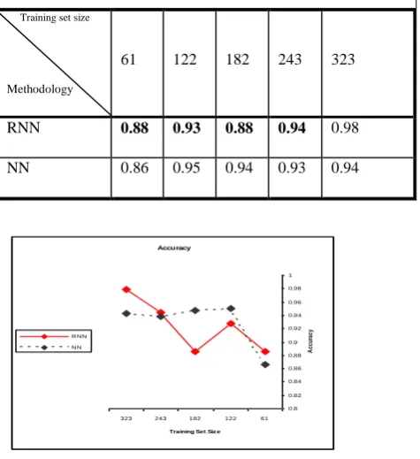
Table 2: RNN and NN accuracy for different data set sizes
Training set size
Methodology
61 122 182 243 323
RNN 0.88 0.93 0.88 0.94 0.98
NN 0.86 0.95 0.94 0.93 0.94
5.
Conclusion
Rough Boundaries are a very good way to handle uncertainty in medical data classifications. The rough neural networks are simulations to human thinking in terms of lower and upper boundaries of the rough set. Instead of one neuron to each input, the rough neural network formats a pair of lower and upper neurons in the input layer. There are input weight for the lower and an other for the upper . The weights are updated during training to represent the lower and upper boundaries of the input value and hence we do not need to prepare rough data for training. The input data is multiplied by the input weights and hence turned into the lower and upper input boundaries of the lower and upper neurons respectively. The hidden layer is also composed of rough neurons. Each rough neuron's pair is fully connected by virtual connections to facilitate information exchange. The lower and upper neurons in the input and hidden layer are fully connected (lower to lower and upper to upper). The hidden rough neurons (lower and upper) produce only one output for each pair and one connecting weight to the output layer which is a single ordinary neuron that tells the network decision
This paper shows that the ability of Rough Neural Networks to learn and classify the medical data can be used as a medical diagnostic system that simulates the human thinking in deciding the accurate output for the input data records of the breast cancer data set. The resulting rough neural network structure of the training phase is further tested by means of testing data set to make sure that the accuracy meets the effective levels of performance. The experiment results are shown and they proved that the proposed model is efficient
than ordinary neural networks applied by the weka rapid miner software for different training data set sizes.
6.
REFERENCES
[1] G. Smolinski, Mariofanna G. Milanova and Aboul-Ella Hassanien Tomasz. 2011. Studies in Computational Intelligence :Computational Intelligence in Biomedicine and Bioinformatics. Springer-Verlag, ISBN-10: 354070776X | ISBN-13: 978-3540707769.
[2] Ger Devlin. 2010. Decision Support Systems Advances in. InTech. ISBN 978-953-307-069-8.
[3] Philip C Jackson. 1985. Introduction to artificial intelligence. New York : Dover worldcat.org. ISBN 048624864X.
[4] Kenji Suzuki. 2011. Artificial Neural Networks: Methodological Advances and Biomedical Applications. InTech. ISBN-13: 9789533072432.
[5] Lingras P. J. 1996. Rough neural network . In: Proc. of the 6th Int. Conf. on Information Processing and Management of Uncertainty in Knowledge-based Systems (IPMU96), Granada, Spain,pp.1445-1450.
[6] Aboul Ella Hassanien. 2006. Rough Neural Intelligent Approach for Image Classification: A Case of Patients with Suspected Breast Cancer. International Journal of Hybrid Intelligent System, IOS press.
[7] Pal S.K. Polkowski S.K. and Skowron A. 2002. Rough-Neuro Computing: Techniques for Computing with Words. Berlin: Springer-Verlag.
[8] Peters J.F. Liting H. and Ramanna S. 2001. Rough Neural Computing in Signal Analysis. Computational Intelligence. Volume 17. no.3. pp. 493-513.
[9] Peters, J.F. Andrzej Skowron, Liting H. and Ramanna S. 2000. Towards Rough Neural Computing Based on Rough Membership Functions: Theory and Application. Rough Sets and Current Trends in Computing. pp. 611-618
[10]A.E. Hassanien, A. Abraham, J.F. Peters and G. Schaefer . 2008. An overview of rough-hybrid approaches in image processing. In proceeding of IEEE International Conference on Fuzzy Systems.
[11] Frank Chiang and Robin Braun . 2004. Intelligent Failure Domain Prediction in Complex Telecommunication Networks with Hybrid Rough Sets and Adaptive Neural Nets,in 3rd international information and telecommunication technologies symposium, Sao Carlos Federal University.
[12]Zhi Xiao, Shi-Jie Ye, Bo Zhong and Cai-Xin Sun. 2009. BP neural network with rough set for short term load forecasting. Expert Systems with Applications . Volume 36 ,Issue 1. pp 273–279.
[13] Roman W. Swiniarski. 1998. Rough Sets and Neural Networks Application to Handwritten Character Recognition by Complex Zernike Moments. RSCTC '98 Proceedings of the First International Conference on Rough Sets and Current Trends in Computing. Springer-Verlag London, UK. pp. 617-624. ISBN:3-540-64655-8.
Accuracy
0.8 0.82 0.84 0.86 0.88 0.9 0.92 0.94 0.96 0.98 1
61 122 182 243 323
Training Set Siz e
A
cc
ur
ac
y
R N N N N
[14]Hongjian Liu, Hongya Tuo and Yuncai Liu. 2004. Rough Neural Network of Variable Precision. Neural Processing Letters. Volume 19 Issue 1,Pages 73 – 87.
[15]Pawlak Z. 1982. Rough Sets. Int. J. Computer and Information Sci. Volume 11, pp. 341–356,
[16]Pawlak Z. Grzymala-Busse J. Slowinski R. and Ziarko W. 1995. Rough sets. Communications of the ACM, Volume 38, no. 11. pp. 89-95.
[17]Z. Pawlak. 1991. Rough Sets: Theoretical Aspects of Reasoning About Data. Kluwer Academic Publishing. Dordrecht.
[18]E.Baum and D.Huassler. 1989. what size net gives valid generalization . Neural Computation . pp 151-160.
[19]http://wiki.pentaho.com/display/DATAMINING/CfsSub setEval.
[20]R. Dechter and J. Pearl. 1985. Generalized Best-First Search Strategies and the Optimality of A*. Journal of the Association for Computing Machinery. pp 505-536.
[21]Russell, Stuart J., Norvig, Peter . 2003. Artificial Intelligence: A Modern Approach (2nd ed.). Upper Saddle River, New Jersey: Prentice Hall. pp. 111–114, ISBN 0-13-790395-2.
[22]http://archive.ics.uci.edu/ml/.