An Asymptotic Distribution Function of the Three Dimensional Shifted van der Corput Sequence

http://dx.doi.org/10.4236/am.2014.515227

An Asymptotic Distribution Function of the

Three-Dimensional Shifted van der Corput

Sequence

Jana Fialová

1

, Ladislav Mišk

2

, Oto Strauch

1

1_{Mathematical Institute, Slovak Academy of Sciences,Bratislava, Slovakia} 2_{Department of Mathematics, University of Ostrava, Ostrava, Czech Republic}

Email: [email protected], [email protected], [email protected]

Received 25 May 2014; revised 1 July 2014; accepted 15 July 2014

Copyright © 2014 by authors and Scientific Research Publishing Inc.

This work is licensed under the Creative Commons Attribution International License (CC BY). http://creativecommons.org/licenses/by/4.0/

Abstract

In this paper, we apply the Weyl’s limit relation to calculate the limit

( ) (

) (

)

(

)

(

)

(

)

,

∑

1

∫ ∫ ∫

1 1 1

0 0 0 0

1

, 1 , 2 , , d d d , ,

lim

N

q q q x y z

N _n

F n n n F x y z g x y z

N

−

→∞ ₌

γ

γ

+

γ

+ =

where γq

( )

n is the van der Corput sequence in base q, g x y z

(

, ,

)

is the asymptotic distribution

function of

(

γ

_q

( ) (

n ,

γ

_q n+1 ,

) (

γ

_q n+2

)

)

, and F x y z

(

, ,

)

=max

(

x y z, ,

)

, min

(

x y z, ,

)

and xyz, re-

spectively.

Keywords

Sequences, Arithmetic Means, Riemann-Stieltjes Integraion

1. Introduction

In this paper we apply the Weyl’s limit relation [1] (p. 1-61)

( )

_{[ ]0,1}

( ) ( )

1

1

d ,

lim N

s n N _n

f f g

N

→∞

∑

₌ x =

∫

x x (1.1)

q and g x

( )

is the asymptotic distribution function (abbreviated a.d.f.) of x_n and s=3. The van der Corput sequence in base q is defined as follows: Let k ₀

k

n=n q ++n be the q-adic expression of a positive integer n. Then

( )

0 1

2 1, 0,1, .

k

q k

n n n

n n

q q q

γ = + + +_{ +} = _ (1.2) It is well-known that this sequence is uniformly distributed (abbreviated u.d.), see [1] (2.11, p. 2-102), [2]

(Theorem 3.5, p. 127), [3] (p. 41).

For s=2 a motivation for the study of the distribution function (abbreviated d.f.) g x y

(

,

)

of

( ) (

)

(

γ

_q n ,

γ

_q n+1

)

, n=0,1, is a result of Pillichshammer and Steinerberger in [4] which states that

( )

(

)

(

)

1

2 0

2 1

1

1 ,

lim N

q q

N _n

q

n n

N γ γ q

−

→∞ ₌

−

− + =

∑

(1.3)

while in J. Fialová and O. Strauch [5] the relation (1.3) was proved applying (1.1) as

(

)

(

)

1 1

2 0 0

2 1

d , q .

x y g x y q

−

− =

∫ ∫

Moreover, in the Unsolved Problems [6] (1.12), the following problem is stated: Find the d.f.

(

1, 2, , s

)

g x x  x of the sequence

(

γ

_q

( )

n ,,

γ

_q

(

n s+ −1

)

)

, n=0,1, 2,, in

[ ]

0,1s. Ch. Aistleitner and M. Hofer [7] gave the following theoretical solution:

Theorem 1 Let

T

denote the von Neuman-Kakutani transformation described in Figure 1. Define the s-

dimensional curve

{

γ

( )

t t; ∈

[

0,1

)

}

, where

γ

( )

t =

(

t T t T,

( ) ( )

, 2 t ,,Ts−1

( )

t

)

. Then the searched a.d.f. is

(

1, 2, , s

)

{

[ ]

0,1 ;

( )

[

0, 1

] [

0, 2

]

[

0, s

]

}

,

g x x  x = t∈ γ t ∈ x × x × × x

where X is the Lebesgue measure of a set

X

.

[image:2.595.204.427.449.717.2]

The paper consists of the following parts: After definitions (Part 2) we derive the a.d.f. of

(

γ

_q

( ) (

n ,

γ

_q n+1

)

)

Figure 1. Line segments containing

(

γq

( ) (

n ,γq n+1

)

)

1, 2,

Haoshangban (Part 3), the a.d.f. of

(

γ

q

( ) (

n ,

γ

q n+2

)

)

(Part 4), intervals containing

( ) (

) (

)

(

γ

q n ,

γ

q n+1 ,

γ

q n+2

)

in diagonals (Part 5) and an explicit form of a.d.f. g x y z

(

, ,

)

(Part 6). As an application (Part 7) we compute the limit

( ) (

) (

)

(

)

(

)

(

)

(

)

1 _{1 1 1}

0 0 0 0

1

, 1 , 2 , , d d d , ,

lim N

q q q x y z

N _n

F n n n F x y z g x y z

N

γ

γ

γ

−

→∞

∑

₌ + + =

∫ ∫ ∫

(1.4)

for F x y z

(

, ,

)

=max

(

x y z, ,

)

, min

(

x y z, ,

)

and xyz, respectively, see (0.39), (0.41) and (0.46).

2. Definitions and Notations

Let x_n, n=1, 2, be a sequence in the unit interval

[

0,1 . Denote

)

•

( )

#

{

; n

[ )

0,

}

N

n N x x

F x

N

≤ ∈

=

the step distribution function (step d.f.) of the finite sequence x₁,,xN in

[

0,1 , while

)

FN

( )

1 =1. • A function g: 0,1

[ ] [ ]

→ 0,1 is a distribution function (d.f.) if

(i) g x

( )

is nondecreasing; (ii) g

( )

0 =0 and g

( )

1 =1.

• A d.f. g x

( )

is a d.f. of the sequence x_n, n=0,1, 2, if an increasing sequence of positive integers

1, 2,

N N  exists such that limk→∞F_Nk

( )

x =g x

( )

a.e. on

[ ]

0,1 .

• A d.f. g x

( )

is an asymptotic d.f. (a.d.f.) of the sequence xn, n=1, 2, if limN→∞F_Nk

( )

x =g x

( )

a.e. on

[ ]

0,1 .

• The sequence x_n is uniformly distributed (abbreviating u.d.) if its a.d.f. is g x

( )

=x.

• Similar definitions take place for s=2, 3 and s-dimensional sequence x_n, n=0,1, 2,, in

[

0,1

)

s, cf. [1] (1.11, pp. 1-60).

• In the sequel the 3-dimensional interval I we denote by I =I_X× ×I_Y I_Z, where IX,IY,IZ are pro- jections on X Y Z, , axes, respectively.

3. a.d.f. of

(

γ

_q

( ) (

n

,

γ

_q

n

+

1 ,

)

)

n

=

1, 2,



Let q≥2 be an integer.

Lemma 1 Every point

(

γ

_q

( ) (

n ,

γ

_q n+1

)

)

, n=0,1, 2,, lies on the diagonals of intervals

1 1

0,1 ,1

q q

 ₋  _× 

   

    (1.5)

1 1

1 1 1 1

1 _i,1 _{i i} , _i , i 1, 2,

q q+ q+ q

   

− − × =

   

     (1.6)

Proof. Express an integer n in the base q

1

1 1 0,

k k

k k

n=n q +n₋q − ++n q+n

where n_i<q and nk >0. We consider the following two cases:

0 0

1 . n < −q 1,

0 0

2 . n = −q 1. Let

0 0

1 . n < −q 1 Then

0

k k

2337

0

1 k k 1

n+ =n q ++n + and by (0.2)

(

)

( )

1

1 q n q n

q

γ + −γ = . In this case

( )

0

1 2

2 1 1

. k

q k

n n q q q

n

q q q q q

γ = + +_{ +} ≤ − + − +_= −

Thus such

(

γ

q

( ) (

n ,

γ

q n+1

)

)

lies on the line-segment

1 1

, 0,1 .

Y X X

q q

 

= + ∈_{ − }

  (1.7) Let

0 0

2 . n = −q 1 Then

(

)

(

)

(

)

1 1

1

1

1

1

k i i i

k i

n

=

n q

+ +



n q

₊ +

+ −

q

q

+ −

q

q

−

+ + −



q

and ni+₁< −q 1, where i=0,1, 2,. Then

(

)

1 1

1

1

k k i

1

i

0

i

0

i

0

n

+ =

n q

+ +



n

+

+

q

+

+ ⋅ + ⋅

q

q

−

+ +



. Thus

( )

1

1 2 1

1 1 i k

q i i k

n n

q q

n

q q q q

γ +

+ + +

− −

= + +_ + + +_ ,

(

)

1

2 1

1

1 i k

q i k

n n

n

q q

γ +

+ +

+

+ = + + , and we have

(

)

( )

2 2 1

1 1 1 1 1 1

1 1 1

q q i i i i

q

n n

q q

q q q q

γ + −γ = ₊ − − _ + + + _= ₊ − + ₊

   and

( )

1 1

1 1 1

1 i i q

q q

n q

q+ q+ γ

− −

− = + + ≤ and

( )

1 2 3 2

1 1 2 1 1

1

q i i i i

q q q q

n

q q q q q

γ ≤ − + + −₊ + −₊ + −₊ += − ₊ . Thus such

(

γ

_q

( ) (

n ,

γ

_q n+1

)

)

lies on the segment

1 2 1 2

1 1 1 1

1 _{i i} , 1 _i ,1 _i , 0,1, 2,

Y X X i

q+ q+ q+ q+

 

= − + + ∈ −_ − _ =

   (1.8)

Thus, for 10, terms of the sequence

(

γ

q

( ) (

n ,

γ

q n+1

)

)

lie on the diagonal of the interval

1 1

: 0,1 ,1

X Y

I I

q q

   

× =_ − _{ }× _

    (1.9) and for 20, after reduction

(

i+ →1

)

i, terms of the sequence

(

γ

_q

( ) (

n ,

γ

_q n+1

)

)

lie on the diagonals of the intervals

( ) ( )

1 1

1 1 1 1

: 1 ,1 , , 1, 2,

i i

X Y i i i i

I I i

q q+ q+ q

   

× = −_ − _{ }× _ =

     (1.10)

These intervals are maximal with respect to inclusion.

Adding the maps (1.7) and (1.8) we found the so-called von Neumann-Kakutani transformation

[ ] [ ]

: 0,1 0,1

T → , seeFigure 1. Because γ_q

( )

n is u.d., the sequence

(

γ

_q

( ) (

n ,

γ

_q n+1

)

)

has a.d.f. g x y

(

,

)

of the form1

( )

(

(

[ ] [ ]

)

)

[ ]

[ ]

(

)

(

[ ]

( )

_{[ ]}

( )

)

1

, Project 0, 0, graph

min 0, , 0, min 0, , 0, ,

X

i i

X Y X Y

i

g x y x y T

x I y I x I y I

∞ =

= × ∩

= ∩ ∩ +

∑

∩ ∩ (1.11)

1

(

)

,

where ProjectX is the projection of a two dimensional set to the X-axis. The sum (1.11) implies

( )

( )

(

) (

)

( )

( )

( )

1

0 if , ,

1 1 1 1 if , ,

1

, if , ,

1

1 if , ,

i i

i i

x y A

y x x y x y B

g x y y x y C

q

x x y D

q−

∈ 

 − − − − = + − ∈

 

= − ∈

 

− + ∈

 

(1.12)

1, 2,

i= 

From (1.12) it follows

( )

1

0, if 0, ,

1 1 1

, , if ,1 ,

1 2 1, if 1 ,1 ,

x q

g x x x x

q q q

x x

q

 _∈ 

  

 



 _{ }



=_ − ∈_ − _

 



 _{ }

 − ∈ −_{ }

 _{ }



(1.13)

and for q=2, the mean equality misses.

4. a.d.f. of

(

γ

_q

( ) (

n

,

γ

_q

n

+

2 ,

)

)

n

=

1, 2,



Let q≥3 be an integer.

Lemma 2 All terms of the sequence

(

γ

_q

( ) (

n ,

γ

_q n+2

)

)

, n=0,1, 2,, lie in the diagonals of the following intervals

2 2

0,1 ,1 ,

q q

 ₋  _× 

   

    (1.14)

1 1

1 1 1 1 1 1

1 _i,1 _{i i} , _i ,i 1, 2, ,

q q

q q+ q+ q

   

− − × + + =

   

     (1.15)

1 1

1 1 1 1 1 1

1 _k,1 _{k k} , _k ,k 1, 2, ,

q q q q+ q+ q

   

− − − − × =

   

     (1.16)

Proof. Express an integer n in the base q

1

1 1 0,

k k

k k

n=n q +n₋q − ++n q+n (1.17) where n_i<q and nk >0. We consider three following cases:

0 0

1 . n < −q 2,

0 0

2 . n = −q 2,

0 0

3 . n = −q 1. Let

0 0

1 . n < −q 2 Then

0

k k

n=n q ++n ,

0

2 _k k 2

(

)

( )

2 1

q n q n q

γ + −γ = . In this case

( )

0

1 2

3 1 2

0 k ,

q k

n n q q q

n

q q q q q

γ ₊ − − −

≤ = + +_ < + +_= and thus such

(

γ

_q

( ) (

n ,

γ

_q n+1

)

)

lies on the

line-segment

2 2

, 0,1 .

Z X X

q q

 

= + ∈_{ − }

  (1.18) Let

0 0

2 . n = −q 2. Then

(

)

(

)

(

)

1 1

1

1

1

2

k i i i

k i

n

=

n q

+ +



n q

+ +

+ −

q

q

+ −

q

q

−

+ + −



q

and ni+1< −q 1, then

(

)

1 1

1

2

_k k _i

1

i

0.

i

0.

i

0

n

+ =

n q

+ +



n

+

+

q

+

+

q

+

q

−

+ +



. Thus

( )

1

1 2 1

2 1 i k

q i i k

n n

q q

n

q q q q

γ +

+ + +

− −

= + +_ + + +_ ,

(

)

1

2 1

1

2 i k

q i k

n n

n

q q

γ +

+ +

+

+ = + +_ , and we have

(

)

( )

2 2 1

1 1 1 1 1 1 1 1

2 1 1

q q i i i i

q

n n

q q q q

q q q q

γ + −γ = ₊ + − − _ + + + _= ₊ + − + ₊

   .

Furthermore

( )

1 1

1 1 2 1

1 i i q

q q

n

q q

q+ q+ γ

− −

− − = + + ≤ and

( )

1 2 3 2

2 1 2 1 1 1

1

q i i i i

q q q q

n

q q q q q q

γ ≤ − + +_ −₊ + −₊ + −₊ +_= − ₊ − .

Thus in this case

(

γ

q

( ) (

n ,

γ

q n+2

)

)

lies on the line-segment

1 2

1 2

1 1 1

1,

1 1 1 1

1 ,1 , 0,1, .

i i

i i

Z X

q q q

X i

q q q q

+ +

+ +

= + + + −

 

∈ − −_ − − _ =

  

(1.19)

Let 0 0

3 . n = −q 1. Then

(

)

(

)

(

)

1 1

1

1

1

1

k i i i

k i

n

=

n q

+ +



n q

₊ +

+ −

q

q

+ −

q

q

−

+ + −



q

and ni+₁< −q 1, then

(

)

1 1

1

2

_k k _i

1

i

0.

i

0.

i

1

n

+ =

n q

+ +



n

₊

+

q

+

+

q

+

q

−

+ +



. Thus

( )

1

1 2 1

1 1 i k

q i i k

n n

q q

n

q q q q

γ +

+ + +

− −

= + + + + + ,

(

)

1

2 1

1 1

2 i k

q i k

n n

n

q q q

γ +

+ +

+

+ = + + +_ , and we have

(

)

( )

2 2 1

1 1 1 1 1 1 1 1

2 1 1

q q i i i i

q

n n

q q q q q q q q

γ + −γ = + ₊ − − _ + + + _= ₊ + − + ₊

   .

( )

1 1

1 1 1

1 i i q

q q

n q

q+ q+ γ

− −

− = + +_ ≤ and

( )

1 2 3

2

1 1 2 1

1 1

q i i i

i

q q q q

n

q q q q

q

γ _{+ + +}

+

− − − −

≤ + + + + +

= −

 

.

This gives

1 2

1 2

1 1 1

1,

1 1

1 ,1 , 0,1, .

i i

i i

Z X

q q q

X i

q q

+ +

+ +

= + + + −

 

∈ −_ − _ =

  

(1.20)

Summary, if the n satisfies 10, then

(

γ

_q

( ) (

n ,

γ

_q n+1

)

)

is contained in the diagonal of

2 2

: 0,1 ,1

X Z

I I

q q

   

× =_ − _{ }× _

    (1.14) for 20 in the diagonal of

( ) ( )

1 1

1 1 1 1 1 1

: 1 ,1 , , 1, 2, ,

i i

X Z i i i i

I I i

q q

q q+ q+ q

   

× = −_ − _{ }× + + _ =

     (1.15)

and for 30 in the diagonal of

( ) ( )

1 1

1 1 1 1 1 1

: 1 ,1 , , 1, 2, ,

k k

X Z k k k k

J J k

q q q q + q + q

   

× = − −_ − − _{ }× _ =

     (1.16).

Proof. Express an integer n in the base q

1

1 1 0,

k k

k k

n=n q +n₋q − + + n q+n (1.17) where n_i<q and nk >0. We consider three following cases:

0 0

1 . n < −q 2, 0 0

2 . n = −q 2, 0 0

3 . n = −q 1. Let

0 0

1 . n < −q 2 Then n=n q_k k+ + n₀, n+ =2 n q_k k+ + n₀+2 and q

(

n 1

)

q

( )

n 2 q

γ + −γ = . In this case

( )

0

1 2

3 1 2

0 k ,

q k

n n q q q

n

q q q q q

γ ₊ − − −

≤ = + + < + += and thus such

(

γ

q

( ) (

n ,

γ

q n+1

)

)

lies on the line-

segment

2 2

, 0,1 .

Z X X

q q

 

= + ∈_{ − }

  (1.18) Let

0 0

2 . n = −q 2. T h e n n n qk k n qi₁ i1

(

q 1

)

qi

(

q 1

)

qi1

(

q 2

)

+ −

+

= + +_ + − + − + +_ − a n d ni+₁< −q 1, t h e n

(

)

1 1

1

2 k k i 1 i 0. i 0. i 0

n+ =n q + + n+ + q+ + q + q− + + . Thus

( )

1 12 1

2 1 i k

q i i k

n n

q q

n

q q q q

γ +

+ + +

− −

= + +_ + + +_ ,

(

)

1

2 1

1

2 i k

q i k

n n

n

q q

γ +

+ +

+

+ = + +_ , and we have

(

)

( )

2 2 1

1 1 1 1 1 1 1 1

2 1 1

q q i i i i

q

n n

q q q q

q q q q

γ + −γ = ₊ + − − _ + + + _= ₊ + − + ₊

Furthermore

( )

1 1

1 1 2 1

1 i i q

q q

n

q q

q+ q+ γ

− −

− − = + +_ ≤ and q

( )

2 i₁1 i ₂2 i ₃1 1 1i ₂ 1

q q q q

n

q q q q q q

γ ≤ − + +_ −₊ + −₊ + −₊ +_= − ₊ − . Thus in this case

(

γ

_q

( ) (

n ,

γ

_q n+1

)

)

lies on the line-segment

1 2 1 2

1 1 1 1 1 1 1

1, 1 ,1 , 0,1, .

i i i i

Z X X i

q q+ q+ q q+ q q+

 

= + + + − ∈ − −_ − − _ =

   (1.19)

Let

0 0

3 . n = −q 1. then n n qk k n qi₁ i1

(

q 1

)

qi

(

q 1

)

qi1

(

q 1

)

+ −

+

= + + + − + − + + − and ni+₁< −q 1, then

(

)

1 1

1

2 k k i 1 i 0 i 0 i 1

n+ =n q + + n+ + q+ + ⋅ + ⋅q q− + + . Thus

( )

1

1 2 1

1 1 i k

q i i k

n n

q q

n

q q q q

γ +

+ + +

− −

= + +_ + + +_ ,

(

)

1

2 1

1 1

2 i k

q i k

n n

n

q q q

γ +

+ +

+

+ = + + + , and we have

(

)

( )

2 2 1

1 1 1 1 1 1 1 1

2 1 1

q q i i i i

q

n n

q q q q q q q q

γ + −γ = + ₊ − − _ + + + _= ₊ + − + ₊

   .

Furthermore

( )

1 1

1 1 1

1 i i q

q q

n q

q+ q+ γ

− −

− = + + ≤ and q

( )

1 i₁1 i ₂2 i ₃1 1 1i ₂

q q q q

n

q q q q q

γ ≤ − + + −₊ + −₊ + −₊ += − ₊ . This gives

1 2 1 2

1 1 1 1 1

1, 1 ,1 , 0,1, .

i i i i

Z X X i

q q+ q+ q+ q+

 

= + + + − ∈ −_ − _ =

   (1.20)

Summary, if the n satisfies 10, then

(

γ

q

( ) (

n ,

γ

q n+1

)

)

is contained in the diagonal of

2 2

: 0,1 ,1

X Z

I I

q q

   

× =_ − _{ }× _

    (1.14), for 20 in the diagonal of

( ) ( )

1 1

1 1 1 1 1 1

: 1 ,1 , , 1, 2, ,

i i

X Z i i i i

I I i

q q

q q+ q+ q

   

× = −_ − _{ }× + + _ =

     (1.15)

and for 30 in the diagonal of

( ) ( )

1 1

1 1 1 1 1 1

: 1 ,1 , , 1, 2, ,

k k

X Z k k k k

J J k

q q q q + q + q

   

× = − −_ − − _{ }× _ =

     (1.16).

Composition of the maps (0.18), (0.19) and (0.20) of Z X

( )

forms the second iteration T2 of the von Neumann-Kakutani transformation T X

( )

. The diagonals of (1.14), (1.16) and (1.15) yield the following graph of T2 inFigure 2.

Here the interval 1 2,1 1

q q

 

− _{− }



  on

X

-axis is decomposed in 1

1 1 1 1

1 _k ,1 _k

q q q q +

 

− − − −

 

 , k=1, 2,, and

the interval 1 1,1 q

 

− _



  is decomposed in 1

1 1

1 _i,1 _i

q q+

 

− −

 

 , i=1, 2,. On

Z

-axis the interval

1 0,

q

 

 

  is

decomposed in 1_{k 1}, 1_k q + q

 

 

 , k=1, 2, and the interval

1 2 , q q

 

 

  is decomposed in 1

1 1 1 1

, i i q q+ q q

 

+ +

 

1, 2,

i= . Note that for q=2, the interval 0,1 2 2,1

q q

 ₋  _× 

   

    has a zero length and is missing.

Exchange for a moment the axis

Z

by

Y

. Similarly as in (1.11), we have that the a.d.f. g x y

(

,

)

of the sequence

(

γ

q

( ) (

n ,

γ

q n+2

)

)

is

( )

(

[ ]

[ ]

)

(

[ ]

( )

_{[ ]}

( )

)

[ ]

( )

_{[ ]}

( )

(

1

)

1

, min 0, , 0, min 0, , 0,

min 0, , 0, .

i i

X Y X Y

i

k k

X Y

k

g x y x I y I x I y I

x J y J

∞ = ∞

=

= ∩ ∩ + ∩ ∩

+ ∩ ∩

∑

∑

(1.21)

[image:9.595.211.420.234.693.2]

Decompose

[ ]

0,12 as the following figure shows: Then byFigure 3 we have

Figure 2. Straight lines containing

( ) (

)

(

γq n ,γq n+2

)

, n=0,1, 2,.

Figure 3.Decomposition of the Vunit square to parts

( )

( )

( )

( )

( )

( )

( )

( )

( )

( )

( )

( )

( )

( )

0 0 0 0 0 0

1

if , ,

2

if , ,

0 if , ,

1 if , ,

2

1 if , ,

if , ,

0 if , ,

1

1 if , ,

,

1 1

1 if , ,

1

if , ,

1

if , ,

1 if , ,

1 1

1 if ,

i i

i i

i

x x y D

y x y C

q

x y A

y x x y B

x x y E

q

y x y F

x y A

x y x y B

q g x y

x x y D

q q

y x y C

q

x y A

q

x y x y B

x x y D

q q

+

∈

− ∈

∈

+ − ∈

− + ∈

∈ ′ ∈

′

+ − + ∈

=

′

− + + ∈

′

− ∈

′′ ∈

′′

+ − ∈

′′

− + + ∈

( )

1

, 1

if , .

i

i i

y x y C

q+                               

 _{− ∈ ′′}



(1.22)

Let q=2.

In this case we find a.d.f g x y

(

,

)

from (1.22) omitting D₀ = C₀ = A₀ = B₀ =0. In Part 7. Applications we need to find g x x

( )

, from g x y

(

,

)

in (1.22):

For q=2

( )

1

0 if 0, ,

4

1 1 1

2 if , ,

2 4 2

,

1 1 3

if , ,

2 2 4

3

2 1 if ,1 .

4 x

x x

g x x

x

x x

 _∈ 

 _ _



 _{ }

− ∈

 _{ }

  

= 

 

 _{∈ }



 _{ }



   −_{ ∈  }   

(1.23)

For q=3

( )

1

0 if 0, ,

3

1 1 2

, if , ,

3 3 3

2

2 1 if ,1 .

3 x

g x x x x

x x

 _∈ 

 _ _



 _{ }

=_ − ∈_{ }

  

 _{ }

− ∈

 _{ }

  

(1.24)

( )

2

0 if 0, ,

2 2 2

, if ,1 ,

2 2 1 if 1 ,1 .

x q

g x x x x

q q q

x x

q

 _∈ 

  

 



 _{ }



=_ − ∈_ − _

 



 _{ }

 − ∈ −_{ }

 _{ }



(1.25)

Note that for q=4 the term x−2 q is omitted.

5. a.d.f. of

(

γ

_q

( ) (

n

,

γ

_q

n

+

1 ,

) (

γ

_q

n

+

2 ,

)

)

n

=

1, 2,



Let q≥3 be an integer.

Lemma 3 Every point

(

γ

q

( ) (

n ,

γ

q n+1 ,

) (

γ

q n+2

)

)

is contained in diagonals of the intervals

2 1 1 2

0,1 ,1 ,1 ,

I

q q q q

     

=_ − _{ }× − _{ }× _

      (1.26)

( )

1 1 1

1 1 1 1 1 1 1 1

1 ,1 , , , 1, 2, ,

i

i i i i i i

I i

q q

q q+ q+ q q+ q

     

= −_ − _{ }× _{ }× + + _ =

       (1.27)

( )

1 1 1

1 1 1 1 1 1 1 1

1 ,1 1 ,1 , ,

k

k k k k k k

J

q q q q + q q+ q+ q

     

= − −_ − − _{ }× − − _{ }× _

     

1, 2, ,

k=  (1.28) where I =0 if q=2. These intervals are maximal with respect to inclusion.

Proof. Every maximal 3-dimensional interval

I

containing points

(

γ

_q

( ) (

n ,

γ

_q n+1 ,

) (

γ

_q n+2

)

)

will be written as I=I_X× ×I_Y I_Z, where IX,IY,IZ are projections of

I

to the X Y Z, , , axes, respectively. Moreover if γ_q

( )

n ∈I_X then γ_q

(

n+ ∈1

)

I_Y and γ_q

(

n+2

)

∈I_Z. From u.d. of γ_q

( )

n follows that the lengths

X Y Z

I = I = I . Combining intervals (1.5), (1.14), (1.15), (1.16), (1.6) of equal lengths by following Figure 3. We find (1.26), (1.27), and (1.28).

Now, let T be the union of diagonals of (1.27), (1.28) and (1.26). Again, as in (1.11), the a.d.f. g x y z

(

, ,

)

has2 the form

(

, ,

)

ProjectX

(

[ ] [ ] [ ]

0, 0, 0,

)

g x y z = x × y × z ∩T (1.29) and it can be rewritten as

(

)

(

[ ]

[ ]

[ ]

)

[ ]

( )

_{[ ]}

( )

_{[ ]}

( )

(

)

[ ]

( )

_{[ ]}

( )

_{[ ]}

( )

(

)

1

1

, , min 0, , 0, , 0,

min 0, , 0, , 0,

min 0, , 0, , 0, .

X Y Z

i i i

X Y Z

i

k k k

X Y Z

k

g x y z x I y I z I

x I y I z I

x J y J z J

∞ = ∞

=

= ∩ ∩ ∩

+ ∩ ∩ ∩

+ ∩ ∩ ∩

∑

∑

(1.30)

To calculate minimums in (1.30) we can use the followingFigure 4 (here q=3):

As an example of application of (1.30) andFigure 4, we compute g x x x

(

, ,

)

for q≥3 without using the knowledge of g x y z

(

, ,

)

,3

(

)

2

0 if 0, ,

2 2 1

, , if ,1 ,

1 3 2 if 1 ,1 .

x q

g x x x x x

q q q

x x

q

 _∈ 

  

 



 _{ }



=_ − ∈_ − _

 



 _{ }

 − ∈ −_{ }

 _{ }



Proof.

1. Let x 0,1 q

 

∈    .

Then

[ ]

0,x ∩I_Z =0,

[ ]

0,x ∩I_Z( )i =0,

[ ]

0,x ∩I_Y( )k =0, consequently g x x x

(

, ,

)

=0.

2. Let x 1 2, q q

 

∈  

 . Then

[ ]

0,x ∩IZ =0,

[ ]

( )

0,x ∩IYk =0,

[ ]

( )

0,x ∩IZi =0, consequently g x x x

(

, ,

)

=0.

3. Let x 2,1 1

q q

 

∈_ − _

 . Then

[ ]

( )

0,x ∩IXi =0,

[ ]

( )

0,x ∩IYk =0, consequently

(

)

2 1 2 2

, , min 1 , ,

g x x x x x x

q q q q

 

= _ − − − _= −

  .

4. Let x 1 1,1 q

 

∈ −_{ }  . Specify ( )k1

X

x

∈

I

, ( )k1

Y

x

∈

J

. Then

[ ]

0,x ∩IX( )k =0,

[ ]

( )

0,x ∩JYk =0 for k>k1. Thus (1.30) implies

(

)

(

[ ]

( )

_{[ ]}

( )

_{[ ]}

( )

)

[ ]

( )

_{[ ]}

( )

_{[ ]}

( )

(

)

1

1

1 1

1 1

1

1

1 1

1 1

1 1

2 1 1 2

, , min(1 ,1 , ) min 0, , 0, , 0,

min 0, , 0, , 0,

2 1 1 1 1 1 1

1 1

3

k

i i i

X Y Z

i k

k k k

X Y Z

k

k k

i i k k k k

i k

g x x x x x I y I z I

q q q q

x J y J z J

x x x

q q q q q q q

=

=

− −

+ +

= =

= − − − − + ∩ ∩ ∩

+ ∩ ∩ ∩

   

= − + _ − _+ − + + _ − _+ − +

   

=

∑

∑

∑

∑

2. x−

For q=2 we have

(

)

1

0 if 0, ,

2

1 1 3

, , if , ,

2 2 4

3

3 2 if ,1 .

4 x

g x x x x x

x x

 _∈ 

 _ _



 _{ }

=_ − ∈_{ }

  

 _{ }

− ∈

 _{ }

  

(1.32)

6. Explicit Form of

g x y z

(

, ,

)

Let q≥3 be an integer.

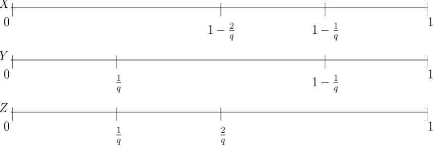
[image:12.595.91.528.96.667.2]

Motivated by theFigure 4 we decompose the unit interval

[ ]

0,1 on

X

,

Y

and

Z

axes in theFigure 5

[image:13.595.91.539.92.249.2]

Figure 5. Divisions of the unit intervals.

intervals (here q=4):

In this decomposition, for

(

x y z, ,

)

∈

[ ]

0,13, we have 27 possibilities. We shall order choices of

(

x y z, ,

)

from the left to the right. Detailed proofs are included only in non-trivial cases.

1. Let

2 1 1

0,1 , 0, , 0,

x y z

q q q

     

∈_ − _ ∈_{ } ∈_{ }

     . Then

(

, ,

)

0 g x y z = .

Proof. We have

[ ]

0,x ∩I( )_Xi =0,

[ ]

0,x ∩J_X( )k =0, i k, =1, 2,. Then, by (1.30),

(

, ,

)

min

(

[ ]

0, X , 0,

[ ]

Y , 0,

[ ]

Z

)

g x y z = x ∩I y ∩I z ∩I .

Similarly, in the following cases 2-9. 2. Let x 0,1 2 ,y 0,1 ,z 0,2

q q q

     

∈_ − _ ∈_{ } ∈_{ }

     . Then

(

, ,

)

0 g x y z = .

3. Let x 0,1 2 ,y 0,1 ,z 2,1

q q q

     

∈_ − _ ∈_{ } ∈_{ }

     . Then

(

, ,

)

0 g x y z = .

4. Let x 0,1 2 ,y 1,1 1 ,z 0,1

q q q q

     

∈_ − _ ∈_ − _ ∈_{ }

     . Then

(

, ,

)

0 g x y z = .

5. Let x 0,1 2 ,y 1,1 1 ,z 1 2,

q q q q q

     

∈_ − _ ∈_ − _ ∈_{ }

     . Then

(

, ,

)

0 g x y z = .

6. Let x 0,1 2 ,y 1,1 1 ,z 2,1

q q q q

     

∈_ − _ ∈_ − _ ∈_{ }

     . Then

) 2 , 1 , ( min = ) , , (

q z q y x z

y x

7. Let x 0,1 2 ,y 1,1 1 ,z 0,1

q q q q

     

∈_ − _ ∈_ − _ ∈_{ }

     . Then

(

, ,

)

0 g x y z = .

8. Let x 0,1 2 ,y 1,1 1 ,z 1 2,

q q q q q

     

∈_ − _ ∈_ − _ ∈_{ }

     . Then

(

, ,

)

0 g x y z = .

9. Let x 0,1 2 ,y 1 1,1 ,z 2,1

q q q

     

∈_ − _ ∈ −_{ } ∈_{ }

     . Then

(

)

2

, , min ,

g x y z x z

q

 

= _ − _

 .

Proof. We use z 2 1 2

q q

− ≤ − .

10. Let x 1 2,1 1 ,y 0,1 ,z 0,1

q q q q

     

∈ −_ − _ ∈_{ } ∈_{ }

     . Then

(

, ,

)

0 g x y z = .

Proof. We use

[ ]

0,x ∩I_X( )i =0,

[ ]

0,y ∩J_Y( )k =0,

[ ]

0,z ∩IZ =0. Similarly,

11. Let x 1 2,1 1 ,y 0,1 ,z 1 2,

q q q q q

     

∈ −_ − _ ∈_{ } ∈_{ }

     . Then

(

, ,

)

0 g x y z = .

12. Let x 1 2,1 1 ,y 0,1 ,z 2,1

q q q q

     

∈ −_ − _ ∈_{ } ∈_{ }

     . Then

(

, ,

)

0 g x y z = .

Proof. We use

[ ]

0,x ∩I_X( )i =0,

[ ]

0,y ∩J_Y( )k =0,

[ ]

0,y ∩J_Y =0.

13. Let x 1 2,1 1 ,y 1,1 1 ,z 0,1

q q q q q

     

∈ −_ − _ ∈_ − _ ∈_{ }

     . Then

(

, ,

)

0 g x y z = .

14. Let x 1 2,1 1 ,y 1,1 1 ,z 1 2,

q q q q q q

     

∈ −_ − _ ∈_ − _ ∈_{ }

     . Then

(

, ,

)

0 g x y z = .

15. Let x 1 2,1 1 ,y 1,1 1 ,z 2,1

q q q q q

     

∈ −_ − _ ∈_ − _ ∈_{ }

     . Then

(

)

1 2

, , min ,

g x y z y z

q q

 

= _ − − _

 .

16. Let x 1 2,1 1 ,y 1 1,1 ,z 0,1

q q q q

     

∈ −_ − _ ∈ −_{ } ∈_{ }

     .

Specify ( )k1

X

x

∈

J

, ( )k2

Y

y

∈

J

, ( )k3

Z

(

)

(

)

3 3 3

3 3

3 3

1 2 3

3 1 2

1

3 1 2

1

3 2 1

1

3 1 2

3

0 if min , ,

1 1 1 1

min 1 , 1 , if ,

1 1 1

min 1 , if ,

1 1

, , _{min 1 , if ,}

1

1 if ,

1

min 1 , 1 if

k k k

k k

k k

k k k

x y z k k k

q q q q

x z k k k

q q q

g x y z _{y z k k k}

q q

z x k k k

q

z x y k k

q

+

+

+

<

 

− + + − + − = =

 

 

 

− + + − = <

 

 

 

= _{ − + −  = <}

 

+ − + < <

 

+ _ − + − _ <

  1 2

3 2 1

,

1 if .

k

z y k k k

              

 ₌

 

+ − < <



Proof. First observe that

[ ]

0,z ∩IZ =0, and

[ ]

( )

0,x ∩I_Xi =0. Thus

[ ]

[ ]

[ ]

(

)

min 0,x ∩I_X , 0,y ∩I_Y , 0,z ∩I_Z =0 and

(

[ ]

( )

[ ]

( )

[ ]

( )

)

1min 0, , 0, , 0, 0.

i i i

X Y Z

i x I y I z I

∞

= ∩ ∩ ∩ =

∑

Further, for k=1, 2,, we have

[ ]

( )

1

1 1

1 1

0 if ,

1 1

0, 1 if ,

1 1

if ; k

X k

k k

k k

x J x k k

q q

k k q q +



 _>



 _{ }



∩ = − − −_ _ =

 

 

 − <



[ ]

( )

2

2

2

2 1

0 if ,

1

0, 1 if ,

1 1

if ; k

Y k

k k

k k

y J x k k

q

k k q q+



 _>



  



∩ =_ − −_{ } =

 

 

− <

 

[ ]

( )

3

3

3 1

3 1

0 if ,

1

0, if ,

1 1

if ; k

Z k

k k

k k

z J z k k

q

k k

q q

+ +



 _>

 

∩ =_ − =

 

− <

 

Thus, using (1.30), we find

(

)

(1 2)

(

_{[ ]}

( )

_{[ ]}

( )

_{[ ]}

( )

)

3

min , =

, , k k min 0, _Xk , 0, _Yk , 0, _Zk k k

g x y z =

∑

x ∩J y ∩J z ∩J .

17. Let x 1 2,1 1 ,y 1 1,1 ,z 1 2,

q q q q q

     

∈ −_ − _ ∈ −_{ } ∈_{ }

     .

Specify ( )k1 X

x∈J , ( )k2 Y

(

)

1 2

1 2

1 2

2 1

min 1 , 1 if ,

2

, , 1 if ,

1

1 if .

x y k k

q q

g x y z x k k

q

y k k

q

  

− + − + =

  

 

 

=_ − + <

 

− + >

 

Proof. We have

[ ]

0,x ∩IX( )i ,

[ ]

0,z ∩IZ ,

[ ]

( )

1

1 1

0,z JZk k k

q q+

∩ = − , then

(

)

_{( )}

(

[ ]

( )

_{[ ]}

( )

)

1 2

min ,

, , _{k k k} min 0, _Xk , 0, _Yk .

g x y z =

∑

_≤ x ∩J y ∩J

18. Let x 1 2,1 1 ,y 1 1,1 ,z 2,1

q q q q

     

∈ −_ − _ ∈ −_{ } ∈_{ }

     .

Specify ( )k1

X

x

∈

J

, ( )k2

Y

y

∈

J

. Then

(

)

1 2

1 2

1 2

2 1 2

min 1 , 1 if ,

, , 1 if ,

1

1 if .

x y z k k

q q q

g x y z x z k k

y z k k

q

  

− + − + + − =

  

 



=_ + − <



 + − − >

 Proof. We have

(

)

_{( )}

(

[ ]

( )

_{[ ]}

( )

_{[ ]}

( )

)

1 2

min ,

2 2 2

, , min 1 ,1 , k k k min 0, Xk , 0, Yk , 0, Zk .

g x y z z x J y J z J

q q q ≤

 

= _ − − − _+ ∩ ∩ ∩

 

∑

19. Let x 1 1,1 ,y 0,1 ,z 0,1

q q q

     

∈ −_{ } ∈_{ } ∈_{ }

     . Then

(

, ,

)

0 g x y z = .

20. Let x 1 1,1 ,y 0,1 ,z 1 2,

q q q q

     

∈ −_{ } ∈_{ } ∈_{ }

     .

Specify ( )i1

X

x

∈

I

, ( )i2

Y

y

∈

I

, ( )i3

Z

z

∈

I

. Then we have

(

)

(

)

1 1 1

1 1

1 1

1 2 3

3 2 1

1 1

3 2 1

3 2 1

1

2 3 1

1

2 3

0 if max , ,

1 1 1 1

min 1 , , if ,

1

min , 1 if ,

1 1

, , min 1 , if ,

1 1 1

min 1 , if ,

1

1 if

i i i

i i

i i

i i i

x y z i i i

q

q q q

y z x i i i

q

g x y z x y i i i

q q

x z i i i

q

q q

x z i i

q

+ +

+

+

<

 

− + − − − = =

 

 

 

− + − = <

 

 

 

= _ − + − _ < =

 

 

− + − − < =

 

 

+ − − < < 1

3 2 1

,

1 if .

i

x y i i i

                 

+ − < <