ARABIC TEXT CLUSTERING BASED ON K MEANS ALGORITHM WITH SEMANTIC WORD EMBEDDING

2973

EFFECT OF CLUSTERING DATA IN IMPROVING MACHINE

LEARNING MODEL ACCURACY

SAMIH M. MOSTAFA1_{, HIROFUMI AMANO}2

1_{Mathematics Department, Faculty of Science, South Valley University, Qena, Egypt} 2_{Research Institute for Information Technology, Kyushu University, Japan}

E-mail: 1 _{[email protected],} 2 _{[email protected]}

ABSTRACT

Supervised machine learning algorithms consider the relationship between dependent and independent variables rather than the relationship between the instances. Machine learning algorithms try to learn the relationship between the input and output from the historical data in order to attain precise predictions about unseen future. Conventional foretelling algorithms are usually based on a model learned and trained from historical data. The instances in the historical data may vary in its characteristics. The variation may be a result of difference in case's pertinence degree to some cases compared to others. However, the problem with such machine learning algorithms is their dealing with the whole data without considering this variation. This paper presents a novel technique to the trained model to improve the prediction accuracy. The proposed method clusters the data using K-means clustering algorithm, and then applies the prediction algorithm to every cluster. The value of K which gives the highest accuracy is selected. The authors performed comparative study of the proposed technique and popular prediction methods namely Linear Regression, Ridge, Lasso, and Elastic. On analysing on five datasets with different sizes and different number of clusters, it was observed that the accuracy of the proposed technique is better from the point of view of Root Mean Square Error (RMSE), and coefficient of determination 𝑅 .

Keywords

:

1. INTRODUCTION

Machine learning (ML) is considered as the important subfield of artificial intelligence and is being adopted for numerous of various applications [1, 2]. ML addresses the study and construction of models capable of learning from the data. Understanding what and how the ML algorithm is learning is an issue for the developers of the ML applications [3]. ML can be classified into unsupervised and supervised. Unsupervised learning groups the data into categories depending on the basis of the similarities between data in each group. On the other hand, supervised learning means that the machine learns with the assistance of the labeled training data. Estimating unknown (independent, dependent) mapping of a system using a specific number of (independent, dependent) samples is called learning [4, 5]. This process of estimating needs data collected (i.e., training data), and an algorithm that deals with this data and learns from it. Generally speaking, the learning algorithm learns pattern in the data on hand and create a set of rules to map input/output

relation. Data is categorized into labeled (with outcome) or unlabeled (without outcome). Outcome variable(s) may be continuous or distinct, regression is a way of predicting for continuous outcome, and classification is a way of predicting for distinct outcome (i.e., the response to be predicted is the probability or the true of an event/class), the number of classes can be two or more. On the other hand, clustering is applied to unlabeled data using the similarities between observations to group them intoclusters [6–8]. The statistical method depends on the characteristics of the data (e.g., similarities between instances in the clustering technique), in other words, the more similarities the better statistical method accuracy. Regression is one of the most common statistical processes for estimating dependent/independent relationship when the dependent to be predicted is a continuous value. The regression line is a refined outline of averages and is drawn in such a way as to reduce the error of the fitted values in relation to the actual values. Equation of the simple linear regression can be defined by the following form:

2974 where C is the intercept and the C is the slope of the regression line. In addition to explaining the relationship between dependent d and independent I variables, the model also predicts the value of dependent variable from the independent variable values from the equation:

d C C I

the hat symbol refers to the predicted value of the unknown coefficient/variable. In simple regression, for a given dependent variable there is one independent variable. However, in real cases there is more than one independent variable, so existing of multiple independent variables is called multivariate regression. The mathematical notation can take the form:

d C I C I C I ⋯ C I

where m is the number of independent variables.

1.1. Goodness of the Model

The performance of the model can be evaluated using following metrics:

• R-squared: how well the model fits the data. •Root Mean Square Error (RMSE): how close the estimated values are to the actual values.

1.2. Paper Contributions & Novelty

This paper gives a brief discussion of machine learning types, proposes a method for improving the prediction accuracy, and compares between the proposed method and the common methods. In contrast to other techniques, e.g., Clustering Lasso (CL) which selects groups of variables that have the same mechanism of predicting the dependent variable [9], the novelty of the proposed work boils down in benefiting from similarities between instances and applying the selected prediction algorithm for each cluster. The proposed work does not depend on collinearity among variables or the number of variables compared to instances.

1.3. Organization

The rest of this paper is organized as follows: Section 2 presents the proposed method

supported with an illustrative example; dataset specification, the prediction algorithms used in the comparison, the parameters used in the comparison, results and discussion are discussed in section 3.

2. PROPOSED METHOD

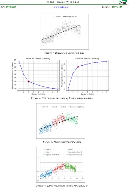
In the proposed method, the authors avail from the similarity attribute of the data by clustering it into groups (clusters) before applying the statistical method. In the proposed method, the number of clusters is determined by the elbow method (heuristic method of validation and interpretation of symmetry within cluster analysis). The data is clustered using K-means algorithm in which the number of clusters resulted from the elbow method is used for the clustering. The selected prediction algorithm is applied for every cluster. For deeper clarification, the next subsection discusses an illustrative example.

Algorithm: Proposed method 1. Input data

2. Select the prediction algorithm 3. Find the value of K using elbow method 4. Cluster the data using K-means

5. Apply the selected prediction algorithm in each cluster

In the proposed method, clustering prepressing step is applied to the data before applying the prediction algorithm for the purpose of improving the accuracy of model generated by the user-selected prediction algorithm.

2.1 Illustrative Example

2975

Figure 1. Regression line for all data

Figure 2. Determining the value of k using elbow method.

Figure 3. Three clusters of the data

Figure 4. Three regression lines for the clusters

2976

3. EXPERIMENTAL IMPLEMENTATION 3.1. Datasets

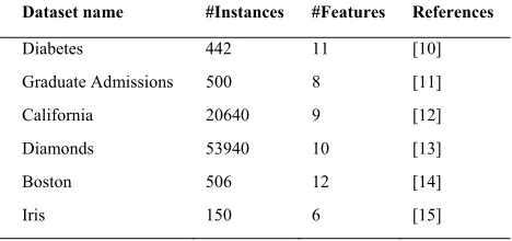
Six datasets that are commonly used in databases repository are used in the comparative study (Table 1).

3.2. Prediction Algorithms

The comparison is done between four common prediction algorithms namely multible linear regression (MLR), Ridge, Lasso, and ElasticNet and the proposed method. Table 2 gives short descriptions of the prediction algorithms used.

Table 1. Datasets specifications

Dataset name #Instances #Features References

Diabetes 442 11 [10]

Graduate Admissions 500 8 [11]

California 20640 9 [12]

Diamonds 53940 10 [13]

Boston 506 12 [14]

Iris 150 6 [15]

Table 2. Packages and functions used

Prediction method Short description References

MLR minimizes the residual sum of squares between the observed responses in the dataset, and the responses predicted by the linear approximation. [16] Ridge solves a regression model where the loss function is the linear least squares function,

and imposes a penalty on the size of the coefficients.

[17]

Lasso estimates sparse coefficients. Coefficients that add lightweight value to the model will be zero

[18]

ElasticNet allows for learning a sparse model where few of the weights are non-zero like Lasso, while still maintaining the regularization properties of Ridge. [19]

3.3. Performance Measure

The comparisons were done from the point of view of the following parameters:

 Root mean squared error (RMSE): indicates how close the forecasted values are to the actual values; hence the lower value of RMSE, the good of the model performance [20]. The mathematical notation can be written as:

𝑅𝑀𝑆𝐸 ∑ 𝑦 𝑦

𝑛

where 𝑦and 𝑦 are the actual value and forecasted value of the i-th observation respectively, and n is the number cases.

 Coefficient of determination (R2 _{score): it is a}

measure of how perfectly the evaluated regression line of the model adapts the data distribution [21]. It can be written as:

𝑅 𝑦, 𝑦 1 ∑_∑ 𝑦 𝑦 𝑦 𝑦 ;

𝑦 1

𝑛 𝑦

3.4. Experimental Results and Discussion

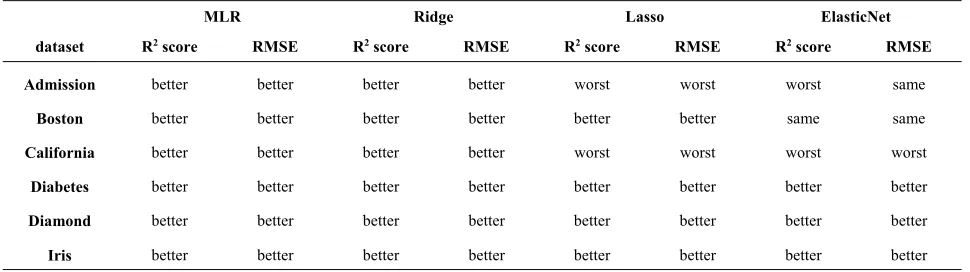
The experiments are conducted on a computer equipped with 16 GB of RAM, Intel core i5-2400 (3.10 GHz), 1 TB of HDD, Gnu/Linux Fedora 28 of OS, and Python (version 3.7) of programming language. Table 3 summarizes the observations by comparing the improvements of the proposed approach versus common four algorithms from the point of view of R2 _{score and}

RMSE. The notable observations are:

 Clustered MLR is better than MLR in R2

score and RMSE for all datasets.

 Clustered Ridge is better than Ridge in R2

score and RMSE for all datasets.

2977 somewhat similar to Lasso for Admission, Boston, and California.

 Clustered ElasticNet is better than ElasticNet for Iris, Diamond, and Diabetes, and behaves somewhat similar to ElasticNet for Admission, Boston, and California

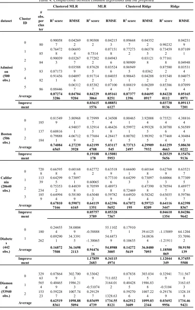
Table 4 shows the comparisons between the four common methods and the proposed method from the point of view of R2 _{score and RMSE.}

Table 3. Proposed approach versus MLR, Ridge, Lasso, and ElasticNet

4. Conclusion and Future Works

This paper introduces a method that aims to improve the prediction accuracy of the model by clustering the data and applying the selected algorithm, which is a user choice, for each cluster. Unlike the traditional supervised algorithms which find the relationship between the dependent and independent variables, the proposed approach benefits from the similarities between the instances

to improve the prediction accuracy. Four common algorithms are compared with the proposed method, the results showed that the proposed method achieves significant improvement from the point of view of RMSE, and coefficient of determination 𝑅 . In the future research avenues, the proposed approach will be analysed in more dataset, other standard error metrics will be considered (e.g., P-value and T-value).

MLR Ridge Lasso ElasticNet

dataset R2 _{score RMSE R}2 _{score RMSE R}2 _{score RMSE R}2 _{score RMSE}

Admission better better better better worst worst worst same

Boston better better better better better better same same

California better better better better worst worst worst worst

Diabetes better better better better better better better better

Diamond better better better better better better better better

2978

Table 4. Comparisons between common algorithms and the proposed

Clustered MLR MLR Clustered Ridge Ridge

dataset Cluster _ID # obs. per clus ter

R2 _{score RMSE R}2 _{score RMSE R}2 _{score RMSE R}2 _{score RMSE}

Admissi on (500 obs.)

0 ₈₀ 0.90058₇ 0.04269₂ 0.90308₂ 0.04215₃ 0.89668₇ 0.04352_{2 0.90232} 0.04231₉ 1

85

0.76472 8

0.06693

4 0.7314

0.07151 8 0.77273 2 0.06578 5 0.73459 2 0.07109 1 2 84 0.90039 3 0.03267 7 0.77202 2 0.04943

6 0.90909

0.03121 8

0.77161

8 0.04948 3 _{83 0.87173} 0.03588₉ 0.87628₅ 0.03524₆ 0.86949_{5 0.0362} 0.87580₂ 0.03531₄ 4 82 0.91456 1 0.04097 6 0.91714 2 0.04035 3 0.90643 1 0.04288 2 0.91548 2 0.04075 5 5 _{86 0.88446} 0.06312₇ 0.85382₇ 0.07100₄ 0.88819₃ 0.06209₉ 0.85386₆ 0.07099₄

Average 0.87274

3286 0.04704 9204 0.84229 3064 0.05161 8251 0.87377 1396 0.04695 0917 0.84228 0112 0.05165 8971 Improve ment 0.03615 1576 0.08851 6127 0.03738 8136 0.09113 7201 Boston (506 obs.)

0 ₁₈₅ 0.81549₉ 3.80968₁ 0.75999₇ 4.34508₄ 0.80465₁ 3.92008₄ 0.75521₄ 4.38816₄ 1

137 0.60816

4.94037 1 0.32914 5 6.46426 8 0.59972 1 4.99328 5 0.30788 6 6.56589 4 2 184 0.79888 1 4.06712 9 0.77684 2 4.28417 4 0.80702 5 3.98392 5 0.77468 4 4.30484 3

Average 0.74084

6565 4.27239 3928 0.62199 4708 5.03117 545 0.73713 2497 4.29909 7932 0.61259 4663 5.08630 0222 Improve ment 0.19108 178 0.15081 5953 0.20329 5656 0.15476 9136 Califor nia (20640 obs.)

0 720₈ 0.66595₈ 0.60168₆ 0.62772₂ 0.63518₉ 0.66600₁ 0.60164₈ 0.62768₉ 0.63521₇ 1 113₃₉ 0.64299₅ 0.73097_{1 0.60065} 0.77310₆ 0.64299₃ 0.73097₃ 0.60066₃ 0.77309₅ 2 ₂₃₄ 0.75353₂ 0.44839₈ 0.70599₁ 0.48973_{8 0.72469} 0.47390₈ 0.70594₇ 0.48977₅ 3 185₉ 0.64994₄ 0.58180₉ 0.63040₂ 0.59782₉ 0.64920₄ 0.58242₄ 0.63035₅ 0.59786₇ Average 0.67810₇₁₆₆ 0.59071₆₁₆₅ 0.64119₁₃₅₁ 0.62396₅₆₅₂ 0.67072₁₉₅ 0.59723₈₂₀₉ 0.64116₃₄₄₇ 0.62398₈₃₆₇

Improve ment 0.05757 3789 0.05328 7367 0.04610 1354 0.04286 9642 Diabete s (442 obs.) 0 180 0.24455 4 38.0004

9 -0.58888

55.1102 7

0.17910

1 39.6125 -1.15089 64.1204 1 ₂₆₂ 0.09290₁ 34.3391_{5 -1.30065} 54.6873_{9 0.10635} 34.0836_{4 -1.21911} 53.7096₂

Average 0.16872₇₅₀₈ 36.1698₂₁₁₃ -0.94476

16

54.8988

3005 0.142725619 36.84807093 -1.18500 069 58.9150 139 Improve ment 1.17859 2683 0.34115 4974 1.12044 349 0.37455 5508 Diamon d (53940 obs.)

0 329

63 0.87864 9 302.700 3 0.33042

9 711.032

0.87838 1 303.034 5 0.32941 9 711.567 8

1 565

4

0.40465 9

1986.21

3 -0.51074

3164.01 2

0.40428 5

1986.83

8 -0.5104

3163.65 3 2 153₂₃ 0.59228₇ 1007.74₂ 0.29129_{7 1328.63} 0.59270₆ 1007.22₄ 0.29176₉ 1328.18₈

Average 0.62519

2979

Improve

ment 15.89965597 0.366475484 15.92727726 0.366358189

Iris (150 obs.) 0 53 0.58589 2 0.15982 4 0.53837 3 0.16874 5 0.60948 6 0.15520 4 0.58034 6 0.16089 1 1 ₉₇ 0.50539₃ 0.24685₁ 0.51907₃ 0.24341₄ 0.50930₆ 0.24587₃ 0.51660₃ 0.24403₈

Average 0.54564

2513 0.20333 7645 0.52872 2806 0.20607 9331 0.55939 6339 0.20053 8486 0.54847 4215 0.20246 4357 Improve ment 0.03200 1092 0.01330 4032 0.01991 3651 0.00951 2148

Clustered Lasso Lasso _ElasticNet Clustered ElasticNet

dataset Cluster _ID # obs. per clus ter

R2 _{score RMSE R}2 _{score RMSE R}2 _{score RMSE R}2 _{score RMSE}

Admissi on (500 obs.)

0 ₈₀ 0.39724₈ 0.10512₃ 0.10319₂ 0.12822₇ 0.624298₈₂₅ 0.08299₅ 0.476870₂₆ 0.09793₄ 1 ₈₅ 0.41897₅ 0.10518₆ 0.21894₆ 0.12195₅ 0.558337₄₁₈ 0.09170₈ 0.500034₇₄₃ 0.09757₃ 2 84 -0.01393 0.10425 7 0.24701 5 0.08984 5 0.590989 869 0.06621 7 0.636564 741 0.06241 9 3 _{83 0.04289} - 0.10233₃ 0.28481₆ 0.08474₃ 0.383689₆₇₈ 0.07866₇ 0.595595₁₅₅ 0.06372₄ 4 ₈₂ 0.21780₂ 0.12398₃ 0.29519_{4 0.11769} 0.653176₁₂ 0.08255₈ 0.645685₈₄ 0.08344₅ 5

86

0.25962 2

0.15979

9 0.29872

0.15552 3 0.649727 827 0.10991 4 0.667472 07 0.10709 3

Average 0.20613

7182 0.11678 0231 0.24131 3579 0.11633 0496 0.576703 29 0.08534 2992 0.587037 135 0.08536 4642 Improve ment -0.14577 048 -0.00386 601 -0.017603 393 0.00025 3615 Boston (506 obs.)

0 ₁₈₅ 0.50421₁ 6.24507₉ 0.63127₆ 5.38567₈ 0.555916₂₀₅ 5.91047₁ 0.635021₈₃₇ 5.35825₁ 1 ₁₃₇ 0.49127₇ 5.62918₉ 0.47095₂ 5.74053₇ 0.489438₃₄₂ 5.63935₃ 0.473984₈₈₅ 5.72406₁ 2 184 0.78851 3 4.17063 9 0.64288 7 5.41955 8 0.705213 571 4.92396 2 0.656423 965 5.31584 5 Average 0.59466₇₁₇₂ 5.34830₂₀₅₃ 0.58170₄₉₉₈ 5.51525₇₇₈₇ 0.583522₇₀₆ 5.49126₁₅₈₉ 0.588476₈₉₅ 5.46605₂₄₅₉

Improve ment 0.02228 3071 0.03027 161 -0.008418 664 -0.00461 194 Califor nia (20640 obs.)

0 720

8 0.19451 1 0.93432 8 0.28420 8 0.88077 1 0.398249 064 0.80756 6 0.422555 231 0.79108 8

1 113

39 0.34741 2 0.98828 5 0.29673 2 1.02594 3 0.450214 811 0.90710 8 0.436138 572 0.91864 7 2 234 -0.00836 0.90696 6 0.31536 8 0.74732 9 0.320412 819 0.74457 1 0.486811 721 0.64702 6

3 185

9 0.06335 1 0.95170 1 0.28480 6 0.83161 9 0.325355 782 0.80769 9 0.420265 792 0.74873 2

Average 0.14922

2980 Diabete s (442 obs.) 0 180 0.01644 9 43.3596 7 -1.50228 69.1600 3 0.000281 698 43.7145 8 -3.415714 253 91.8730 2 1 262 -0.02383 36.4817 1 -1.62935 58.4636 8 -0.023699 919 36.4794 7 -2.644023 327 68.8260 4 Average -0.00368 829 39.9206 8967 -1.56581 185 63.8118 5592 -0.011709 111 40.0970 2716 -3.029868 79 80.3495 3014 Improve ment 0.99764 4487 0.37440 0116 0.996135 44 0.50096 7497 Diamon d (53940 obs.)

0 329

63 0.87573 9 306.308 3 0.32562 2 713.579 5 0.743478 863 440.100 9 -0.320155

658 998.397

1 565

4 0.40457 5 1986.35 3

-0.50916 3162.36

0.253176 236 2224.60 1 -2.206191

315 4609.33

2 153

23 0.59348 8 1006.25 7 0.29303 3 1327.00 2 0.402987 813 1219.44 9 0.416165 349 1205.91 6

Average 0.62460

0687 1099.63 9291 0.03649 6857 1734.31 3961 0.466547 637 1294.71 6959 -0.703393 874 2271.21 4188 Improve ment 16.1138 214 0.36595 1428 1.663280 779 0.42994 502 Iris (150 obs.) 0 53 -0.03211 0.25231 8 -6.74515 0.69119 4 -0.032111 237 0.25231 8 -1.973883 919 0.42829 9 1 97 -0.19781 0.38414 9 -0.18902 0.38273 7 -0.197813 953 0.38414 9 0.367240 443 0.27920 6 Average -0.11496 26 0.31823 3686 -3.46708 467 0.53696 541 -0.114962 595 0.31823 3686 -0.803321 738 0.35375 2519 Improve ment 0.96684 1711 0.40734 7886 0.856890 97 0.10040 588 REFERENCES:

[1] T. Segaran, Programming Collective

Intelligence: Building Smart Web 2.0 Applications. 2007.

[2] D. Vallejo-Huanga, P. Morillo, and C.

Ferri, “Semi-Supervised Clustering

Algorithms for Grouping Scientific Articles,” Procedia Comput. Sci., vol. 108, pp. 325–34, 2017.

[3] V. K. Ayyadevara, Pro Machine

Learning Algorithms. 2018.

[4] V. Cherkassky and F. M. Mulier,

Learning from Data : Concepts, Theory, and Methods / V. Cherkassky, F. Mulier. 1998.

[5] W. A. Yousef and S. Kundu, “Learning

algorithms may perform worse with increasing training set size: Algorithm-data incompatibility,” Comput. Stat. Data Anal., vol. 74, pp. 181–97, 2014.

[6] K. Chen and L. Liu, “The ‘Best K’ for

Entropy-based Categorical Data

Clustering.,” 2005, pp. 253–62.

[7] M. N. Murty, P. J. Flynn, and A. K. Jain,

“Data Clustering: A Review,” ACM Comput. Surv., vol. 31, p. 43, 1999.

[8] A. K. Jain and R. C. Dubes, “Algorithms

for Clustering data.” 1988.

[9] Q. Yu and B. Li, “Regularization and

Estimation in Regression with Cluster Variables,” Open J. Stat., vol. 04, no. 10, pp. 814–25, 2014.

[10] N. D. of Statistics, “Diabetes

Data-1-5-2019,” NCSU Department of Statistics.

[Online]. Available:

https://www4.stat.ncsu.edu/~boos/var.sel ect/diabetes.html. [Accessed: 01-May-2019].

[11] M. S. Acharya, “Graduate

Admissions-1-5-2019,” Kaggle Inc, 2018. [Online].

Available:

https://www.kaggle.com/mohansacharya /graduate-admissions. [Accessed: 01-May-2019].

[12] C. Nugent, “California Housing

Prices-3-5-2019,” Kaggle Inc, 2017. [Online].

Available:

https://www.kaggle.com/camnugent/cali fornia-housing-prices. [Accessed: 03-May-2019].

[13] M. Shiva, “Diamonds-20-4-2019,”

2981 https://www.kaggle.com/shivam2503/di amonds. [Accessed: 20-Apr-2019].

[14] I. Kaggle, “Boston Housing-25-4-2019.”

[Online]. Available:

https://www.kaggle.com/c/boston-housing. [Accessed: 25-Apr-2019].

[15] I. Kaggle, “Iris Dataset-25-4-2019.”

[Online]. Available:

https://www.kaggle.com/jchen2186/mac hine-learning-with-iris-dataset. [Accessed: 25-Apr-2019].

[16] D. W. Gareth James Trevor Hastie,

Robert Tibshirani, An introduction to statistical learning : with applications in R. New York : Springer, [2013] ©2013.

[17] Scikit-learn, “Ridgre

Regression-26-4-2019.” [Online]. Available:

https://scikit-learn.org/stable/modules/generated/sklea rn.linear_model.Ridge.html. [Accessed: 26-Apr-2019].

[18] Scikit-learn, “Lasso

Regression-27-4-2019.” [Online]. Available:

https://scikit-learn.org/stable/modules/linear_model.ht ml. [Accessed: 27-Apr-2019].

[19] Scikit-learn, “Elastic Net

Regression-28-4-2019.” [Online]. Available:

https://scikit-learn.org/stable/modules/linear_model.ht

ml#elastic-net. [Accessed:

28-Apr-2019].

[20] I. B. Aydilek and A. Arslan, “A hybrid

method for imputation of missing values using optimized fuzzy c-means with support vector regression and a genetic algorithm,” Inf. Sci. (Ny)., vol. 233, pp. 25–35, 2013.

[21] T. Beysolow II, Introduction to Deep