Full Length Research Article
STANDALONE MICROGRID USING PV ARRAY WITH CSI
*
Pradeepa, S., Hariharan, R. and Ajay, R.
B.M.S. College of Engineering, Bangalore, India
ARTICLE INFO ABSTRACT
In this paper, Photovoltaic (PV) array is connected to a Current Source Inverter (CSI) fed load. The application of solar PV panel output as input to CSI is plating industry. The advantage of the proposed micro-grid is the rumination of DC-DC converter of traditional PV systems. In addition to this, Maximum Power Point Tracking (MPPT) algorithm is also been implemented for generating constant current at the source of CSI.
Copyright © 2014 Pradeepa et al. This is an open access article distributed under the Creative Commons Attribution License, which permits unrestricted use, distribution, and reproduction in any medium, provided the original work is properly cited.
INTRODUCTION
One of the major concerns in the power sector is the day-to-day increasing power demand. The unavailability of enough resources to meet the power demand using the conventional energy sources, has led to renewable energy sources being seen as the future sources capable of providing surplus energy and they are also a cleaner alternative. There is a new vigor being shown in this field in recent decades. Solar is the largest source among all renewable energy sources as sun is the largest energy source available to us. India being a tropical country most of the days are sunny, so solar energy is the most feasible among all renewable energy sources. Photovoltaic (PV) arrays are the most common method used to tap the solar energy and use it in the form of electrical energy. The high cost, low efficiency and dependence on environmental conditions of the PV arrays make them less popular. Mechanical tracking systems are being used to obtain maximum power from them, but more cheaper and efficient methods are being worked out and MPPT (Maximum power point tracking) is one such method. In this paper, the feasibility of interfacing a CSI to a solar panel, in lieu of the conventional VSI, is investigated. The general block diagram of a PV array connected to CSI fed load is as shown in Fig.1.
CSI-Based Modeling of Solar Cell
A solar cell is the building block of a solar panel. A photovoltaic module is formed by connecting many solar cells
*Corresponding author: Pradeepa, S., B.M.S. College of Engineering, Bangalore, India
in series and parallel. Considering only a single solar cell; it can be modeled by utilizing a current source, a diode and two resistors. This model is known as a single diode model of solar cell. Two diode models are also available but only single diode model is considered here (Kalpana et al., 2013; Hairul Nissah Zainudin and Saad Mekhilef, 2010; Liu et al., 2004). The V-I characteristics equation of a solar cell is given by
= − ∗ [exp ∗ ∗
∗ ∗ } − 1 −
∗
(1)
= ∗ ∗ exp ∗ ∗ ∗ (2)
Ilg = {Iscr + Ki ∗ (T − 25)} ∗ lamdba/1000 (3)
The representations used in the above equations are given below.
I &V : Cell output current and voltage; Ios : Cell reverse saturation current; T : Cell temperature in Celsius;
k : Boltzmann's constant=1.38 * 10-23J/K; q : Electron charge=1.6*10-19C;
Ki: Short circuit current temperature coefficient at Iscr=0.065/0C;
lambda : Solar irradiation in W/m2;
Iscr : Short circuit current at 25 degree Celsius=3.8A; Ilg : Light-generated current;
Ego : Band gap for silicon=1.12eV; A : Ideality factor;
ISSN:
2230-9926
International Journal of Development Research
Vol. 4, Issue, 3, pp. 642-646, March,2014
DEVELOPMENT RESEARCH
Article History: Received 08th January, 2014
Received in revised form 11th February, 2014
Accepted 15th February, 2014
Published online 14th March, 2014
Tr : Reference temperature=250C; Ior : Cell saturation current at Tr; Rsh : Shunt resistance;
Rs : Series resistance;
The characteristic equation of a solar module is dependent on the number of cells in parallel and number of cells in series. Thus, the characteristic EQ.1 is changed as given in EQ. 4. These equations are used in modeling the solar cell.
[image:2.595.37.287.170.253.2]= ∗ − ∗ ∗ ∗ ∗ ∗∗ − − ∗ ∗ (4)
Figure 1. Block Diagram representation of PV Array Connected to CSI Fed Load
The typical I-V and P-V curves obtained for the characteristic equations are as shown in Fig.2. In this paper, the PV array model is designed by neglecting the shunt resistance. The values indicated along with the constants are taken for a solar cell whose data sheet is as shown in Table 1.
Fig. 2. I-V and P-V Characteristics
Table 1. Specifications of the solar panel
We have 3 unknowns in the characteristic equations: Rs (series resistance), A (ideality factor) and Ior (Cell saturation current at Tr). These unknowns are calculated from three conditions, namely, short circuit condition (I=Isc amperes, V=0), open circuit condition (I=0 amperes, V=Voc volts) and at maximum power point (I=Imp, V=Vmp). The values of Isc, Voc, Imp and Vmp are obtained from the data sheet (Seok-IL Go et al., 2011). Thus the calculated values are as:
A=1.2 Rs=0.008ohm Ior=2.16*10-8A
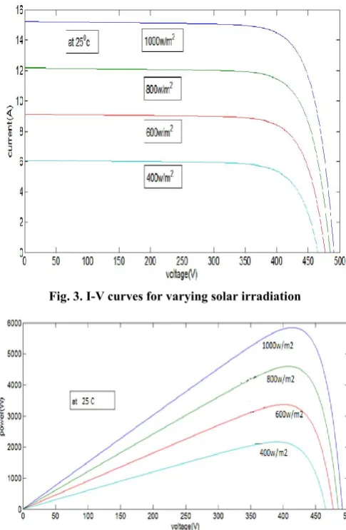
Effect of variation of solar irradiation on panel characteristics
[image:2.595.310.553.284.656.2]The P-V and I-V curves of a solar cell are highly dependent on the solar irradiation values. The solar irradiation as a result of the environmental changes keeps on fluctuating. Higher is the solar irradiation, higher would be the solar input to the solar cell and hence power magnitude would increase for the same voltage value. With increase in the solar irradiation the open circuit voltage increases. This is due to the fact that, when more sunlight incidents on to the solar cell, the electrons are supplied with higher excitation energy, thereby increasing the electron mobility and thus more power is generated (Tarak Salmi et al., 2012). The Fig.3 and Fig.4 are the variation I-V curve and P-V curve for varying solar irradiation respectively.
Fig. 3. I-V curves for varying solar irradiation
Fig. 4. P-V curves for varying solar irradiation
Maximum power tracking algorithms
[image:2.595.52.276.356.501.2]matches with the load impedance. Hence our problem of tracking the maximum power point reduces to an impedance matching problem. In the conventional method, of connecting a Voltage Source Inverter at the output of solar array, it requires a DC/DC converter at its input for regulating the DC source voltage. Hence, a converter is connected to a solar panel in order to enhance the output voltage so that it can be used for different applications like motor load. Whereas, in this case of CSI connected system, especially, where the requirement is being constant current for load applications, it is advantageous to have a solar panel connected to CSI fed loads. There are different techniques used to track the maximum power point. Few of the most popular techniques are:
1) Perturb and observe (hill climbing method) 2) Incremental Conductance method
3) Fractional short circuit current 4) Fractional open circuit voltage 5) Neural networks
6) Fuzzy logic
The choice of the algorithm depends on the time complexity the algorithm takes to track the MPP, implementation cost and the ease of implementation (Trishan Esram et al., 2012; Sangitha et al., 2012; Liu et al., 2004; Seok-IL Go et al., 2011).
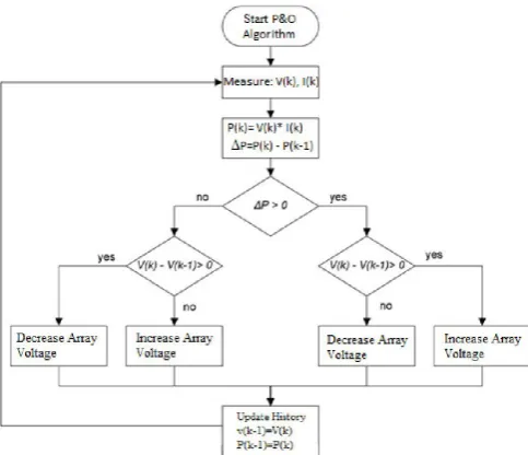
Perturb & Observe
Perturb & Observe (P&O) is the simplest method. In this we use only one sensor, that is the Voltage sensor, to sense the PV array voltage and so the cost of implementation is less and hence easy to implement. The time complexity of this algorithm is very less but on reaching very close to the MPP it doesn’t stop at the MPP and keeps on perturbing on both the directions. When this happens the algorithm has reached very close to the MPP and we can set an appropriate error limit or can use a wait function which ends up increasing the time complexity of the algorithm. However the method does not take account of the rapid change of irradiation level (due to which MPPT changes) and considers it as a change in MPP due to perturbation and ends up calculating the wrong MPP. To avoid this problem we can use incremental conductance method (Mohammed A. Elgendy et al., 2012).
Incremental Conductance
Incremental conductance method uses two voltage and current sensors to sense the output voltage and current of the PV array. At MPP the slope of the PV curve is 0.`
(dP/dV)MPP=d(VI)/dV (5)
0=I+VdI/dVMPP (6)
dI/dVMPP = - I/V (7)
The left hand side is the instantaneous conductance of the solar panel. When this instantaneous conductance equals the conductance of the solar then MPP is reached. Here we are sensing both the voltage and current simultaneously. Hence the error due to change in irradiance is eliminated. However the complexity and the cost of implementation increases. As we go down the list of algorithms the complexity and the cost of implementation goes on increasing which may be suitable for a highly complicated system. This is the reason that Pertur
band Observe and Incremental Conductance method are the most widely used algorithms. Owing to its simplicity of implementation we have chosen the Perturb & Observe algorithm for our study among the two.
Fractional open circuit voltage
The near linear relationship between VMPP and VOC of the PV array, under varying irradiance and temperature levels, has given rise to the fractional VOC method.
VMPP = k1 Voc (8)
where k1 is a constant of proportionality. Since k1 is dependent on the characteristics of the PV array being used, it usually has to be computed beforehand by empirically determining VMPP and VOC for the specific PV array at different irradiance and temperature levels. The factor k1 MPPT For PV Array has been reported to be between 0.71 and 0.78. Once k1 is known, VMPP can be computed with VOC measured periodically by momentarily shutting down the power converter. However, this incurs some disadvantages, including temporary loss of power.
Fractional short circuit current
Fractional ISC results from the fact that, under varying atmospheric conditions, IMPP is approximately linearly related to the ISC of the PV array.
IMPP =k2Isc (9)
where k2 is a proportionality constant. Just like in the fractional VOC technique, k2 has to be determined according to the PV array in use. The constant k2 is generally found to be between 0.78 and 0.92. Measuring ISC during operation is problematic. An additional switch usually has to be added to the power converter to periodically short the PV array so that ISC can be measured using a current sensor.
Fuzzy Logic Control
Microcontrollers have made using fuzzy logic control popular for MPPT over last decade. Fuzzy logic controllers have the advantages of working with imprecise inputs, not needing an accurate mathematical model, and handling nonlinearity.
Neural Network
Another technique of implementing MPPT which are also well adapted for microcontrollers is neural networks. Neural networks commonly have three layers: input, hidden, and output layers. The number nodes in each layer vary and are user-dependent. The input variables can be PV array parameters like VOC and ISC, atmospheric data like irradiance and temperature, or any combination of these. The output is usually one or several reference signals like a duty cycle signal used to drive the power converter to operate at or close to the MPP.
SIMULATED RESULTS AND DISCUSSION
increment, if the resulting change in power change in P is positive, then we are going in the direction of MPP and we keep on perturbing in the same direction. If change in P is negative, we are going away from the direction of MPP and the sign of perturbation supplied has to be changed. For simulation purpose the irradiation is considered to be 1000 W/m2 at a temperature of 25oC. Figure 5 shows the plot of module output power versus module voltage for a solar panel at a given irradiation. The point marked as MPP is the Maximum Power Point, the theoretical maximum output obtainable from the PV panel.
[image:4.595.313.557.261.434.2]Fig. 5. Solar panel characteristics showing MPP and operating points A and B
Fig. 6. Flowchart of Perturb & Observe algorithm
Consider A and B as the two operating points. As shown in the figure above, the point A is on the left hand side of the MPP. Therefore, we can move towards the MPP by providing a positive perturbation to the voltage. On the other hand, point B is on the right hand side of the MPP. When we give a positive perturbation, the value of change in P becomes negative, thus it is imperative to change the direction of perturbation to achieve MPP. The flowchart for the P&O algorithm is shown in Fig. 6. The mathematical model of the PV array has been implemented. The PV array model which inputs array
temperature (T), incident solar irradiation (lambda or S), number of cells in series (Ns) and number of cells in parallel (Np). The input solar irradiation to the PV array can be either a constant or varying which can be selected by changing the switch. The outputs of PV array are array voltage and current. The system has been modeled using MATLAB/SIMULINK.
Table 2. Parameter value taken for simulation
Array temperature (T in °C) 25 Solar irradiance (S in W/m2) 1000 Number of cells in parallel (Np) 1 Number of cells in series (Ns) 36 Load Resistance (Ro range) 2 – 1ohms.
[image:4.595.310.555.266.640.2]The I-V and P-V curves for the PV array designed are as shown in Fig. 7. and Fig. 8. respectively
Fig. 7. I-V Characteristics
Fig. 8. P-V Characteristics
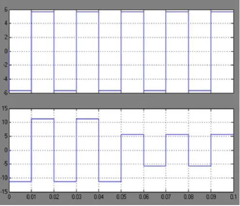
[image:4.595.42.284.436.644.2] [image:4.595.310.554.465.647.2]the input current to CSI and its corresponding output current magnitude remains constant. Whereas the output voltage magnitude varies in proportion to the varying load.
Fig. 9. Reference Current-Input to CSI
Fig. 10. CSI Output Current and Output Voltage
Conclusion
In this paper, it can be observed from the simulated results that for application of CSI fed loads, it requires a constant DC source current at its input. in practice it is difficult to have such a source. And secondly, the importance of renewable
energy sources are shooting up for its own advantages mentioned in the above sections. Having these two factors, in mind, it is verified that solar array connected to CSI fed loads are simple in implementation. It can also been observed that the MPPT algorithm supports in deriving maximum power from the solar array, and generate the corresponding reference current for CSI. It can be taken forward in future to implement a closed loop control for the same tracking system and time varying load.
REFERENCES
Kalpana, SaiBabu, J. Surya Kumar “Design And Implementation Of Different MPPT Algorithms For PV System” International Journal Of Science, Engineering And Technology Research (IJSETR) Vol.2, Issue 10, October 2013”.
Hairul Nissah Zainudin, Saad Mekhilef “Comparison study of Maximum Power Point Tracker techniques for PV systems” Proceedings of the 14th International Middle East power systems conference (MEPCON 2010), Cairo University, Egypt, December 2010, paper id 278.
Liu, C., B. Wu, R. Cheung “Advanced Algorithm for MPPT control of PV systems” Canadian Solar Buildings conference Montreal, August 2004.
Seok-IL Go, Seon- JuAhn, Joon-Ho Choi, Won-Wook Jung, Sang-Yun Yun, IL-Keun Song “Simulation and Analysis of existing MPPT control methods in a PV Generation Systems” Journal of International Council on Electrical engineering vol.1, No.4, 2011.
Tarak Salmi, Mounir Bouzguenda, Adel Gastli, Ahmed Masmoudi “MATLAB/Simulink Based Modelling of Solar Photovoltaic Cell” INTERNATIONAL JOURNAL of RENEWABLE ENERGY RESEARCH, Vol.2, No.2, 2012 Trishan Esram, Patrick L. Chapman “Comparison of
Photovoltaic Array Maximum Power Point Tracking Techniques” IEEE TRANSACTIONS ON ENERGY CONVERSION, VOL. 22, NO. 5. Sangitha S. Kondawar, U.B. Vaidya “A comparison of two MPPT Techniques for PV systems in MATLAB Simulink” International Journal of Engineering Research and Development Volume 2, Issue 7, August 2012.
Sangitha S. Kondawar, U.B. Vaidya “A comparison of two MPPT Techniques for PV systems in MATLAB Simulink” International Journal of Engineering Research and Development Volume 2, Issue 7, August 2012.
Mohammed A.Elgendy, Bashar Zahawi, David J.Atkinson “Assessment of Perturb and Observe MPPT algorithm implementation techniques for PV Pumping Applications” IEEE transactions on sustainable energy, vol.3, number 1, January 2012.
[image:5.595.40.288.320.532.2]