Estimation and testing of persistence in nonlinear and cyclical time series

(1)

T h e E stim a tio n and T estin g o f

P ersisten ce in N on lin ear and

C yclical T im e Series

Violetta Dalla

London School of Economics

July 2006

(2)

UMI Number: U222069

INFORMATION TO ALL USERS

The quality of this reproduction is dependent upon the quality of the copy submitted.

In the unlikely event that the author did not send a complete manuscript and there are missing pages, these will be noted. Also, if material had to be removed,

a note will indicate the deletion.

Dissertation Publishing

UMI U222069

Published by ProQuest LLC 2014. Copyright in the Dissertation held by the Author. Microform Edition © ProQuest LLC.

ProQuest LLC

789 East Eisenhower Parkway P.O. Box 1346

(3)

D eclaration

I hereby declare:

• No part of this doctoral dissertation has been presented to any University for any degree.

• Parts of Chapters 2, 3 and 5 were undertaken as joint work with Professor Javier Hidalgo and Dr Liudas Giraitis.

Violetta Dalla

(4)

n

Libra< v

(5)

A b stract

Throughout this thesis, we are concerned with filling some of the gaps in the lit erature concerning parametric and semiparametric W hittle estimation of long-run and/or cyclical persistence in economic time series. In Chapter 2, we consider local Whittle estimation, and without relying on the assumption of a linear model, we establish sufficient conditions for consistency and provide expansions and rate of convergence for the estimator. In Chapter 3, we apply the results of Chapter 2 to examine the local Whittle estimator for the signal plus noise model and some special cases of it: structural model, nonlinear transformations of a Gaussian process, and long memory stochastic volatility model. Under these specifications, we establish the asymptotic properties of the estimator, and raise several issues concerning its rate of convergence and finite sample bias. In Chapter 4, we employ Monte-Carlo simulations to investigate the finite sample properties of the local W hittle estimator under the linear and nonlinear specifications of Chapters 2 and 3. Furthermore, we apply local Whittle estimation to expected and realized inflation rates, nominal and real interest rates, and transformations of foreign exchange rate returns, in order to assess their long-run persistence and address several issues that have appeared in the empirical literature. Finally, Chapter 5 presents two testing procedures, based on the parametric W hittle method, for the null hypothesis of no persistent compo nent in the data. We derive the asymptotic properties of our test statistics, and moreover introduce and validate a bootstrap scheme for calculating their critical values. A Monte-Carlo study of the finite sample performance of our testing pro cedures, and an empirical application on the growth rate of industrial production and unemployment rate are also included.

(6)

A ck n ow led gem en ts

I would like to thank my supervisor, Professor Javier Hidalgo for his constant pres ence, participation and advice during these years. I will be permanently indepted to him for his generous and invaluable help. I would also like to thank Liudas Giraitis for his advice and assistance. Thanks also to Afonso Gongalves da Silva for his support, and to all my friends and LSE colleagues. Financial assistance through the Greek State Scholarships Foundation (IKY), the ESRC grants R000238212 and R000239936, and the Dennis Sargan Memorial Fund is also gratefully acknowledged. Finally, I would like to thank my parents, Agisilaos and Leoni, my sister, Maria, my grandmother, Marika, and Julian for their encouragement, support and belief.

(7)

C on ten ts

1 Introduction 15

1.1 The notion of persistence... 15

1.2 Quantifying persistence... 16

1.2.1 Long-run p e rsisten c e... 18

1.2.2 Cyclical persistence... 19

1.2.3 C om m ents... 20

1.3 Estimation of persistence... 21

1.3.1 Parametric methods ... 22

1.3.2 Semiparametric m e th o d s... 26

1.4 Description of the t h e s i s ... 28

2 General conditions for local W h ittle estim ation 30 2.1 In tro d u ctio n... 30

2.2 The local Whittle e s tim a to r ... 32

2.3 Assumptions... 34

2.4 Theoretical results on local Whittle estim atio n ... 35

2.4.1 Consistency of the local Whittle e s tim a to r ... 35

2.4.2 Expansions and convergence rate for the local W hittle esti mator 37

2.5 An example: Linear p r o c e s s ... 40

2.6 Final com m ents... 42

2.A A p p e n d ix ... 43

2.B A p p e n d ix ... 60

3 Local W h ittle estim ation for nonlinear tim e series 78 3.1 Introduction... 78

3.2 Signal plus noise p ro c e s s ... 81

3.3 Structural m o d e l ... 86

(8)

3.4 Nonlinear functions of a Gaussian process ... 88

3.5 Long memory stochastic volatility m o d e l... 93

3.A A p p e n d ix ... 97

3.B A p p e n d ix ... 116

4 Local W h ittle estim ation: M onte-Carlo sim ulations and empirical applications 124 4.1 Introduction... 124

4.2 Monte-Carlo sim u latio n s... 126

4.2.1 Linear process... 126

4.2.2 Signed plus noise m o d el... 127

4.2.3 Structural m o d e l ... 129

4.2.4 Nonlinear functions of a Gaussian p r o c e s s ... 130

4.2.5 Long memory stochastic volatility m o d e l... 131

4.3 Empirical a p p lic a tio n s ... 133

4.3.1 Inflation and expected inflation r a t e s ... 133

4.3.2 Nominal and real interest r a t e s ... 136

4.3.3 Exchange r a t e s ... 142

4.A A p p e n d ix ... 146

4.B A p p e n d ix ... 177

5 Param etric bootstrap tests for weak persistence 191 5.1 Introduction... 191

5.2 Test s ta tis tic s ... 193

5.2.1 Wald test Tw ... 194

5.2.2 Lagrange multiplier test Tlm... ... 195

5.3 C onditions... 197

5.4 Statistical properties of Tw and Tl m ... 200

5.5 Bootstrap algorithm for Tw and TL M ... 202

5.6 Monte-Carlo sim u latio n s... 208

5.7 Empirical a p p lic a tio n s... 211

5.7.1 Industrial p ro d u ctio n ... 211

5.7.2 Unemployment r a t e ... 212

5.8 Final com m ents...214

(9)

5.A A p p e n d ix ... 215 5.B A p p e n d ix ... 225 5.C A p p e n d ix ... 230

Bibliography 242

(10)

L ist o f F igures

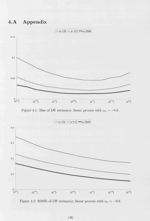
4.1 Bias of LW estimator; linear process with a x = —0.8...146

4.2 RMSE of LW estimator; linear process with a x = —0.8... 146

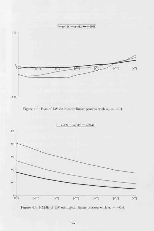
4.3 Bias of LW estimator; linear process with a x = —0.4...147

4.4 RMSE of LW estimator; linear process with a x = —0.4... 147

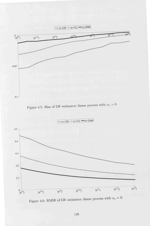
4.5 Bias of LW estimator; linear process with a x = 0... 148

4.6 RMSE of LW estimator; linear process with a x = 0... 148

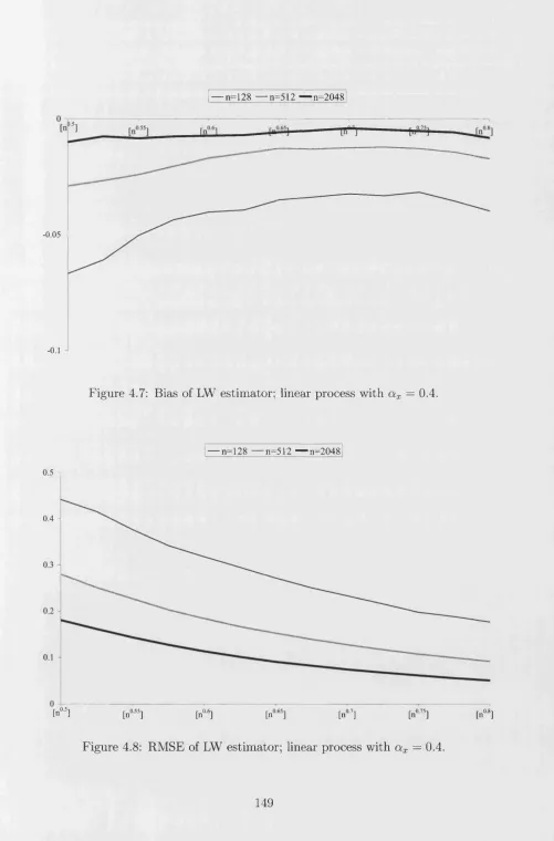
4.7 Bias of LW estimator; linear process with a x = 0.4...149

4.8 RMSE of LW estimator; linear process with a x = 0.4... 149

4.9 Bias of LW estimator; linear process with a x = 0.8...150

4.10 RMSE of LW estimator; linear process with a x = 0.8... 150

4.11 Bias of LW estimator; signal plus noise model with a y = 0.8 and a z = - 0 .8 ... 151

4.12 RMSE of LW estimator; signal plus noise model with a y = 0.8 and = - 0 .8 ... 151

4.13 Bias of LW estimator; signal plus noise model with a y = 0.8 and a* = - 0 .4 ... 152

4.14 RMSE of LW estimator; signal plus noise model with a y = 0.8 and - - 0 .4 ... 152

4.15 Bias of LW estimator; signal plus noise model with a y = 0.8 and a z = 0... 153

4.16 RMSE of LW estimator; signal plus noise model with a y = 0.8 and olz = 0... 153

4.17 Bias of LW estimator; signal plus noise model with a y = 0.8 and = 0.4... 154

4.18 RMSE of LW estimator; signal plus noise model with a y = 0.8 and = 0.4... 154

4.19 Bias of LW estimator; signal plus noise model with a y = 0.8, a z = 0 and signal-to-ratio = 2... 155

4.20 RMSE of LW estimator; signal plus noise model with a y = 0.8, a z = 0 and signal-to-ratio = 2... 155

(11)

4.21 Bias of LW estimator; signal plus noise model with a y = 0.8, a z = 0 and signal-to-ratio = 0.5... 156

4.22 RMSE of LW estimator; signal plus noise model with a y = 0.8,

a z = 0 and signal-to-ratio = 0.5... 156 4.23 Bias of LW estimator; signal plus noise model with a y = 0.8, a z = 0

and p = —0.5... 157

a z = 0 and p — —0.5... 157

4.25 Bias of LW estimator; signal plus noise model with a y = 0.8, a z — 0

and p = 0.5... 158

a z = 0 and p = 0.5... 158 4.27 Bias of LW estimator; structural model with a/ii = 0.4, aUiCx = 0.1

and u — 0.15... 159

4.28 RMSE of LW estimator; structural model with a = 0.4, olu,Cx = 0 .1

and u = 0.15... 159 4.29 Bias of LW estimator; structural model with a^x = 0 .4 , a W)Cl = 0 .3

and uj = 0.15... 160

4.30 RMSE of LW estimator; structural model with a = 0.4, a UyCx = 0.3

and u = 0.15... 160

4.31 Bias of LW estimator; exponential of Gaussian process with ax = 0

and d£ = 0... 161

4.32 RMSE of LW estimator; exponential of Gaussian process with a x = 0

and a£ = 0... 161

4.33 Bias of LW estimator; exponential of Gaussian process with ax = 0.4

and ci£ = 0.4... 162

4.34 RMSE of LW estimator; exponential of Gaussian process with ax =

0.4 and a% = 0.4... 162

4.35 Bias of LW estimator; exponential of Gaussian process with ax = 0.8

and d£ = 0.8... 163

4.36 RMSE of LW estimator; exponential of Gaussian process with dx =

0.8 and = 0.8... 163

4.37 Bias of LW estimator; square of Gaussian process with dx = 0 and

cif = 0... 164

4.38 RMSE of LW estimator; square of Gaussian process with dx = 0 and

ae = 0... 164

4.39 Bias of LW estimator; square of Gaussian process with dx = 0 and

d£ = 0.3... 165

4.40 RMSE of LW estimator; square of Gaussian process with dx = 0 and

d£ = 0.3... 165

(12)

4.41 Bias of LW estimator; square of Gaussian process with ax = 0.4 and

at = 0.7... 166

4.42 RMSE of LW estimator; square of Gaussian process with ax = 0.4

and a,£ = 0.7... 166

4.43 Bias of LW estimator; square of Gaussian process with ax = 0.8 and

d£ = 0.9... 167

4.44 RMSE of LW estimator; square of Gaussian process with ax = 0.8

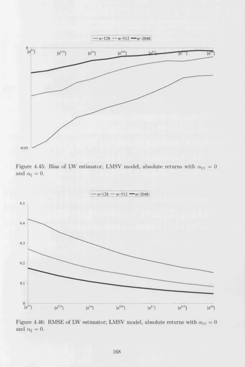
and a,£ — 0.9... 167 4.45 Bias of LW estimator; LMSV model, absolute returns with a |r| = 0

and a£ = 0... 168 4.46 RMSE of LW estimator; LMSV model, absolute returns with ajr| = 0

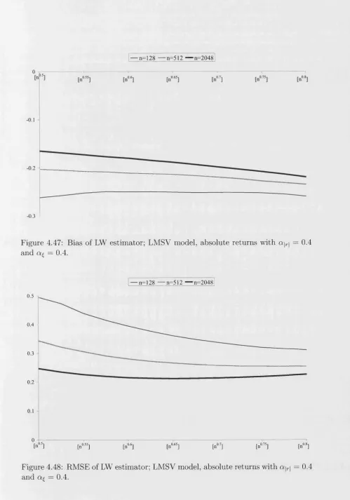
and ct£.... = 0... 168 4.47 Bias of LW estimator; LMSV model, absolute returns with a |r| = 0.4

and ct£ = 0.4... 169 4.48 RMSE of LW estimator; LMSV model, absolute returns with a |r| =

0.4 and a $ = 0.4... 169 4.49 Bias of LW estimator; LMSV model, absolute returns with a |r| = 0.8

and af = 0.8... 170

4.50 RMSE of LW estimator; LMSV model, absolute returns with a\r\ —

0.8 and a $ = 0.8... 170

4.51 Bias of LW estimator; LMSV model, squared returns with ar 2 = 0

and af = 0... 171

4.52 RMSE of LW estimator; LMSV model, squared returns with ar 2 — 0

and ct£ = 0... 171

4.53 Bias of LW estimator; LMSV model, squared returns with ar 2 = 0.4

and af = 0.4... 172

4.54 RMSE of LW estimator; LMSV model, squared returns with ar 2 =

0.4 and af = 0.4... 172

4.55 Bias of LW estimator; LMSV model, squared returns with ar 2 = 0.8

and = 0.8... 173

4.56 RMSE of LW estimator; LMSV model, squared returns with ar 2 =

0.8 and a % = 0.8... 173 4.57 Bias of LW estimator; LMSV model, log-squared returns with aiogr2 =

0 and aif = 0... 174 4.58 RMSE of LW estimator; LMSV model, log-squared returns with

<*iogr2 = 0 and a£ = 0... 174 4.59 Bias of LW estimator; LMSV model, log-squared returns with aiogr2 =

0.4 and = 0.4... 175 4.60 RMSE of LW estimator; LMSV model, log-squared returns with

a iogr2 = 0.4 and a % = 0.4... 175

(13)

4.61 Bias of LW estimator; LMSV model, log-squared returns with a\ o g r 2 =

0.8 and a % = 0.8... 176 4.62 RMSE of LW estimator; LMSV model, log-squared returns with

cqogr2 = 0.8 and af = 0.8... 176 4.63 Data on inflation rate (CPI), inflation rate (GDPDEFL) and ex

pected inflation rate (SPF) for the period 1981Q4-2005Q4...177 4.64 LW estimates for the data in Figure 4.63... 177 4.65 Data on nominal interest rate, inflation rate and ex post real interest

for the period 1954Q3-2005Q4... 178

4.66 LW estimates for the data in Figure 4.65... 178

4.67 Data on nominal interest rate, inflation rate and ex post real interest for the period 1954Q3-1979Q2... 179

4.69 D ata on nominal interest rate, inflation rate and ex post real interest for the period 1979Q3-1987Q2... 180

4.71 Data on nominal interest rate, inflation rate and ex post real interest for the period 1987Q3-2005Q4... 181 4.72 LW estimates for the data in Figure 4.71... 181 4.73 Data on nominal interest rate, expected inflation rate and ex ante

real interest for the period 1987Q3-2005Q4... 182 4.74 LW estimates for the data in Figure 4.73... 182 4.75 Data on nominal interest rate, expected inflation rate, ex ante real

interest and output gap for the period 1987Q3-2005Q4... 183 4.76 LW estimates for the data in Figure 4.75... 183 4.77 Sample autocorrelation function of nominal interest rate, expected

inflation rate, ex ante real interest and output gap for the period 1987Q3-2005Q4... 184 4.78 Periodogram of nominal interest rate, expected inflation rate, ex ante

real interest and output gap for the period 1987Q3-2005Q4...184

4.79 Data on UK£/US$ foreign exchange rate returns rt for the period

1971M2-2006M5... 185

4.80 Data on UK£/US$ foreign exchange rate absolute returns \rt \ for the

period 1971M2-2006M5... 185

4.81 Data on UK£/US$ foreign exchange rate squared returns r\ for the

period 1971M2-2006M5... 186

4.82 Data on UK£/US$ foreign exchange rate quartered returns |r4|5 for the period 1971M2-2006M5... 186

(14)

4.83 Data on UK£/US$ foreign exchange rate log-squared returns log rf for the period 1971M2-2006M5... 187

4.84 LW for UK£/US$ foreign exchange rate absolute returns \rt \, squared

returns r f , quartered returns \rt \* and log-squared returns logr\ for the period 1971M2-2006M5... 187 4.85 Data on JP ¥ /U S $ foreign exchange rate returns rt for the period

1971M2-2006M5... 188

4.86 Data on JP ¥/U S $ foreign exchange rate absolute returns \rt \ for the

period 1971M2-2006M5... 188 4.87 Data on JP ¥/U S $ foreign exchange rate squared returns rf for the

period 1971M2-2006M5... 189

4.88 Data on JP ¥/U S $ foreign exchange rate quartered returns |rt | ^ for the period 1971M2-2006M5... 189

4.89 D ata on JP ¥/U S $ foreign exchange rate log-squared returns log r\

for the period 1971M2-2006M5... 190

4.90 LW for JP ¥ /U S $ foreign exchange rate absolute returns \rt \, squared

returns rf, quartered returns |r*|* and log-squared returns logrf for the period 1971M2-2006M5... 190

5.1 D ata on industrial production for the period 1960M1-2006M5. . . . 238 5.2 Data on growth rate of industrial production for the period 1960M1-

2006M4... 238 5.3 D ata on unemployment rate for the period 1960M1-2006M5... 240 5.4 Data on growth of unemployment rate for the period 1960M1-2006M4.240

(15)

L ist o f Tables

5.1 Size of test; i.i.d. model... 230

5.2 Size of T£M test; i.i.d. model...230

5.3 Size of T£M test; AR(1) model...230

5.4 Size of T£M test; M A (1) model...230

5.5 Power of T ^ test; A R F I M A ( 0 ,0.1,0) model...231

5.6 Power of T ^ test; ARFIM A(Q, 0.2,0) model...231

5.9 Power of T£M test; A R F I M A (0,0.1,0) model... 232

5.10 Power of T£M test; A R F I M A (0,0.2,0) model... 232

5.11 Power ofT£M test; A R F I M A (0,0.3,0) model... 232

5.12 Power of T£M test; A R F I M A ( 0 ,0.4,0) model... 232

5.13 Power of T£M test; G A R M A (0 ,0.1,0) model...233

5.17 Power of T£M test; A R F I M A (1,0.1,0) model...234

5.18 Power of T£M test; A R F I M A ( 1 ,0.2,0) model...234

5.21 Power o£T£M test; G A R M i4(l,0.1,0) model...235

5.22 Power of T£M test; G A R M A (1,0.2,0) model...235

5.25 Power of T£M test; A R F I M A ( 0,0.1,1) model... 236

5.26 Power of T£M test; A R F I M A {0,0.2,1) model...236

5.27 Power of T£M test; A R F I M A (0,0.3,1) model...236

5.28 Power of T£M test; A R F I M A ( 0,0.4,1) model... 236

(16)

5.29 Power of T£M test; G A R M A (0,0.1,1)..model...237

5.31 Power of T£M test; G A R M A (0 ,0.3,1)..model...237

5.32 Power of T£M test; G A R M A (0,0.4,1)..model...237

5.33 and T£M statistics and their bootstrap critical vaules for growth rate of industrial production for the period 1960M1-2006M4...239

5.34 Tw and T£M statistics and their bootstrap critical vaules for growth rate of industrial production for the period 1960M1-1984M3...239

5.35 Tw and T£M statistics and their bootstrap critical vaules for growth rate of industrial production for the period 1984M4-2006M4...239

5.36 T ^ and T£M statistics and their bootstrap critical vaules for unem ployment rate for the period 1960M1-2006M5...241

5.37 T ^ and T£M statistics and their bootstrap critical vaules for unem ployment rate for the period 1960M1-1973M12...241

5.38 Tw and T£M statistics and their bootstrap critical vaules for unem ployment rate for the period 1974M1-1986M2...241

5.39 Tw and T£M statistics and their bootstrap critical vaules for unem ployment rate for the period 1986M3-2006M5...241

(17)

C h ap ter 1

In tro d u ctio n

1.1

T h e notion o f persistence

The persistence property of a time series, defined as the degree of dependence be tween observations in time, is of undoubted interest for several reasons. First, the degree of persistence gives the practitioner an indication of the existence and strength of mean reversion, and as a by-product, of the sensitivity to shocks of the time series under consideration. Second, a correct understanding of the degree of persistence is a crucial step towards building an appropriate model for the dynamics governing the data. Last, but not least, prior knowledge of the level of persistence is essential for performing correct statistical inference, as different degrees of persis tence may give rise to different distributional properties of the same test statistic. Two broad types of persistence are the main focus of this thesis, which we refer to as long-run persistence and cyclical persistence. The former relates to the dependence of observations that are far apart in time, while the latter is concerned with the dependence of observations in the same phase of a cycle.

Numerous empirical studies have found evidence of long-run persistence in macroeconomic and financial time series. It was first pointed out by Granger (1966) that various economic times series, such as industrial production and commodity prices indexes, exhibit strong long-run persistence. Such behaviour has been consequently reported by various authors using different approaches, sample periods and trans formations of the data. Among others, we cite Greene and Fielitz (1977) for stock returns, Nelson and Plosser (1982) for different measures of output, wages, indus trial production, employment, prices, money stock, stock prices and interest rates, Diebold and Rudebusch (1989) for output, Diebold and Rudebusch (1991) for

(18)

ous measures of income, Sowell (1992) for output, Ding, Granger, and Engle (1993) for the S&P500 series, Backus and Zin (1993) for inflation rate, interest rate and money growth, Cheung (1993) for various exchange rates, Ding and Granger (1996) for various stock returns and exchange rates, Baillie, Chung, and Tieslau (1996) for inflation rate, Andersen and Bollerslev (1997) for exchange rates, Gil-Alana and Robinson (1997) for output, industrial production, employment, different mea sures of prices, wages, money stock, velocity, bond yield and stock prices, Lobato and Robinson (1998) for various exchange rates, Lobato and Velasco (2000) for the stock market trading volume, Sun and Phillips (2004) for nominal and real interest rates, inflation and expected inflation rates. In the aforementioned studies, there is an overall agreement that the long-run persistence of the various series examined is strong.

On the other hand, the empirical literature on cyclical persistence is rather lim ited and it is usually concerned with the seasonality of the data. Strong seasonal behaviour has been reported by Arteche and Robinson (2000) for inflation, and by Arteche (2004) for stock index. Nonseasonal cyclical pattern is evident in various macroeconomic time series and is attributed to business cycle behaviour, see King and Watson (1996) for output growth, employment growth, real balance growth, money supply growth, inflation rate, nominal and real interest rate. The persistence of the business cycle component however was not quantified by King and Watson (1996), although the theoretical business cycle literature emphasizes th at the busi ness cycle behaviour is strongly persistent, as deviations from the average level of economic activity are maintained for considerable lengths of time, see for example Diebold and Rudebusch (1999).

1.2

Q uantifying persistence

Suppose that we are interested in analyzing the persistence properties of a covari ance stationary process {xt}tei with mean nx and variance o\. The main tool for

describing dependence in the time domain is the autocovariance function {7x{t)}teZ

given by

7*(t) = E ((zt - f!x) (xt+T - nx) ) . (1.2.1)

In this thesis, we focus on the frequency domain approach. To that end, we assume

further th at {xt}tez has an absolutely continuous spectral distribution function, so

(19)

th at the spectral density function f x(.) of {xt}tez exists, and it is such that

7T

7 .( t) =

J

eM f x(X)d\, (1.2.2)

— 7r

where f x(.) is a non-negative, even and periodic function of period 27T when extended

beyond the range (—7r,7r].

The spectral density function is the main tool in the frequency domain for an alyzing dependence. It is essentially the Fourier transform of the autocovariance function and therefore, the spectral density function captures the same information

about the structure of {xt}tez as the autocovariance function. Since the spectral

density function records the contribution of the components belonging to a given frequency band to the total variation of the process, the decomposition into long-, medium- and short-run comes more naturally, see for example Chapter 7 in Ander son (1971). Notice that the long-run is associated with low frequency components, while a cycle of period Tx corresponds to the frequency u x = jr.

If {xt}tez were a white noise sequence, then it would not exhibit either long-run or cyclical persistence. Notice that for white noise processes, we have 7x(r) = 0 for all t 7^ 0, and f x(A) = c for all A G [0,7r] and some 0 < c < 0 0 . If {xt}tez

followed a covariance stationary Autoregressive Moving Average model of orders p,

q (A R M A (p ,q)), then it is well know that its dependence would be rather weak, resulting to an autocovariance function that is absolutely summable and thus to a spectral density function such that 0 < f x(A) < 0 0 for all A G [0,7r]. White noise

sequences and covariance stationary A R M A(p, q) models fall in the class of weakly

dependent processes.

Here, the concept of weak dependence corresponds to time series that have an autocovariance function, which is absolutely summable. On the other hand, we refer to a time series process being strongly dependent, when its autocovariance function is not absolutely summable. It should be mentioned that the notion of weak/strong dependence is not always associated with summability properties of second moments. For example, Doukhan (1994) and Nze, Biihlmann, and Doukhan (2002) quantify dependence as a measure based on the covariance between func tions of the past and the future. An earlier and similar concept was introduced by McLeish (1975), known as mixingale or general near epoch dependence, which measures how fast the conditional moments converge to the unconditional ones. Stronger concepts are those of strong-mixing, see Rosenblatt (1956), or ^-mixing, see Volkonskii and Rozanov (1959), which are based on the variation norm between

(20)

the joint probability function and the product of their marginal.

1.2.1

Long-run p ersisten ce

A common "local” parameterization of the spectral density function for the purpose of quantifying long-run persistence is

/*(A) ~ cq)X |A| Qi , as A —► 0, (1.2.3)

with — 1 < a x < 1 and 0 < Co,x < oo. Here, the notation ~ means that the ratio of

left and right hand side tends to 1. The parameter a x is referred to as the memory

parameter and it quantifies the degree of long-run persistence of the process {xt}tez-

Notice that for 0 < a x < 1, the spectral density function is unbounded at zero, so that the variation associated with the zero frequency component, i.e. the long-run, is substantial. Actually, the higher the value of the memory parameter, the more of the variation is explained by the long-run component and hence, the stronger the long-run persistence is. This case is usually referred to as {xt}tez having long

memory. For a x = 0, the spectral density function is bounded and bounded away

from zero at the zero frequency. Then, the variation of {x t}tez explained by the

long-run component is not significant, and {xt}tez is said to have short memory.

Hence, white noise sequences and covariance stationary A R M A (p, q) models exhibit

short memory. For — 1 < a x < 0, the spectral density function is equal to zero at the zero frequency, and it is said th at {xt}tez has negative memory. In empirical applications, such a situation is not commonly found in the levels of the data, but arises when the data has been overdifferenced.

The earliest model satisfying (1.2.3) is the fractional noise introduced by Man delbrot and van Ness (1968), whose autocovariance function satisfies

The spectral density function of the fractional noise is complicated, see Sinai (1976), but indeed satisfies (1.2.3).

The most widely used parametric model satisfying (1.2.3) is the Autoregressive Fractionally Integrated Moving Average model of orders p, d, q (A R F I M A ( p, d, q))

introduced by Adenstedt (1974) and explored by Granger and Joyeux (1980). The latter specification is an extension of the Autoregressive Integrated Moving Aver

age of orders p,d,q (A R IM A (p ,d ,q)) model of Box and Jenkins (1976) with the

7* (t ) = ~ (\t +1£*x+ i 2 |7"|Qx"^ + |t —1|°-+1) . (1.2.4)

(21)

parameter d allowed to take noninteger values. Under such a specification, {xt}tez is given by

a(L )(l - L f x t = b(L)st, (1.2.5)

where — | < rf < | is referred to as the differencing parameter, L is the lag operator,

{£t}tez is a white noise sequence, and a(L) and b(L) are the autoregressive and moving average polynomials

a(L) = 1 — a\L — ... — avLP and b(L) = 1 + b\L + ... + bqLq, (1.2.6)

respectively, all of whose zeros lie outside the unit circle and a(L) and b(L) have no

common zeros. Then, the spectral density function is given by

f x W ~ 2;r I I |a(e~a )|2 ’ 7 r < X - * ' (L2-7)

It can be easily shown that (1.2.7) satisfies (1.2.3) with a x = 2d, noticing that 11 — e~lX\ 2d = |2 sin | | 2d and sin A ~ A, as A —► 0.

Finally, we should mention the extension of the exponential model of Bloomfield (1973) considered by Robinson (1994a), whose spectral density function is given by

/x(A) = |l - e“*A| 2dexp ( y , cfc cos ((fc - 1) A)^ , -7r < A < ir. (1.2.8)

Then, one can easily check, as in (1.2.7), that (1.2.8) satisfies (1.2.3) with a x = 2d.

1.2.2

C yclical p ersistence

Cyclical persistence at a known frequency u x ^ {0,7r} is just an extension of the long-run one described in Subsection 1.2.1, as now one needs to be concerned with the frequency ujx instead of the zero one. A "local" parameterization of the spectral

density function for quantifying cyclical persistence is

/x(A) ~ Cq,cj,x |A - Ux \~a“’x, as A u x, (1.2.9)

with — 1 < a UtX < 1 and 0 < Co)CJ)X < oo. We refer to the parameter aU}X as the cyclical memory parameter, which quantifies the strength of the cyclical component. As in the case of long-run persistence, when 0 < aUfX < 1, the spectral density

function is unbounded at the frequency cux. Then, a substantial amount of the

variation of {xt}tez is associated with the cyclical component, and the higher the value of aUiX the stronger the cyclical component is. Hence, for 0 < aUyX < 1

(22)

we say that {xt}tez has long cyclical memory. For a UtX = 0, the spectral density

function is bounded and bounded away from zero at the frequency u x, so that the

cyclical component of {%t}tez is weak. We refer to this case as {xt}tez having short

cyclical memory, and notice that white noise sequences and covariance stationary

A RM A(p, q) models fall in this category. When — 1 < a UjX < 0, the spectral density

function is equal to zero at the frequency u x, and it is said that {xt}tez has negative

cyclical memory. The latter situation is rather uncommon in practical situations, but might arise if the data has been seasonally overdifferenced, that is, a procedure has been applied to the data to extract the seasonal component but the initial strength of the seasonal component had been overestimated.

A parametric model satisfying (1.2.9) is the Gegenbauer Autoregressive Moving

Average model of orders p ,d u,q (G A R M A (p, du, q)) of Gray, Zhang, and Woodward

(1989). Under such specification, {xt}tez is given by

a(L)( 1 — 2 cos (ljx) L -f L2)d“x t = b(L)et, (1.2.10)

where we refer to — \ < du < \ as the cyclical differencing parameter, and a(L),

b(L) and {£t}tez are as defined above in (1.2.5). Then, the spectral density function

is given by

f x W = Tp |l - 2cos(ux)e~lX + | | 2 , -ir < A < 7r. (1.2.11)

lit |a (e -zA)|

It can be easily shown that (1.2.11) satisfies (1.2.9) with = 2du , noticing that

11 — 2 cos(o;a;)e_*A + e-2iA | 2du> = |4 sin sin | 2d and sin A ~ A, as A —► 0.

1.2.3

C om m ents

Notice that models (1.2.3) and (1.2.5) can be considered as special cases of (1.2.9) and (1.2.10) respectively. Hence, the latter specifications can be combined in the case that the nature of the possibly persistent component is not known. One can regard the following "local" specification for the spectral density function

/*(A) ~ Q),io,x |A - ujx \~aw'x, as A —> cjx, (1.2.12)

with — 1 < olu,x < 1, 0 < Co^x < oo and u x G [0,7r ]. On the other hand, when we

are concerned with parametric modelling, we can consider (1.2.10), th at is,

a(L )(l — 2 cos (cjx) L + L2)d“x t = b(L)et, (1.2.13)

(23)

with — \ < du < \ when ujx G (0,7r) and — \ < du < \ when ujx G {0,7r}, while

a(L), b(L) and

{£t}te

z are as defined above in (1.2.5). In both (1.2.12) and (1.2.13),

the frequency ujx is unknown, and therefore, u x can be treated as another parameter

that needs to be estimated.

Before we proceed with overviewing the methods for estimating persistence, there are three points that we need to add. Firstly, we concentrate on covariance

stationary processes, and therefore, we require the parameters a x and to be less

than 1. In practical situations, it is likely that one would encounter data sets with nonstationary characteristics. Here, we assume that appropriate transformations can be applied to the data, so that the resulting series axe covariance stationary with a x and/or a UiX less than 1.

Secondly, the specifications presented in Subsections 1.2.1 and 1.2.2 are not the only parametric models satisfying (1.2.3) and (1.2.9), respectively. For example, (1.2.5) satisfies (1.2.9) with a U)X = 0, while (1.2.3) holds for (1.2.10) with a x = 0.

Furthermore, the ARFIMAijp^d^d^.q) model, see Robinson (1994c) and Giraitis

and Leipus (1995), is given by

o ( i) ( 1 - 2 cos (u .) L + - L)dx t = b(L)et, (1.2.14)

where d, dw, a(L), b(L) and

{et}tez

are as defined above in (1.2.5) and (1.2.10), and satisfies (1.2.3) and (1.2.9) with a x = 2d and = 2du), respectively. Actually, we show in Chapter 3 below, th at various nonlinear models satisfy (1.2.3) and (1.2.9)

such as linear combinations of A R F IM A (p ,d ,q ) and/or GARMA(p, d^, q) mod

els, as well as nonlinear transformations of A R F I M A ( p, d, q) or G A R M A (p, dw, q)

models.

Lastly, when examining cyclical components at a frequency ujx ^ {0,7r}, the

specifications (1.2.9), (1.2.10), (1.2.12), (1.2.13), and (1.2.14) entail the assumption

th at cycles with frequencies just above and below ojx have the same contribution to

the total variation of {

xt}tez

• One could relax such a restriction as it was done in Arteche and Robinson (2000), however we are not going to consider this case here.

1.3

E stim ation o f persistence

As described above, the parameters a x and quantify the long-run and cyclical

persistence of

{xt}te

z>

respectively. Suppose now th at a stretch of data

{xi,

...,

xn}

is available, where n denotes the sample size, and we are interested in performing

(24)

inference on ax and/or a WiI. In this section, we overview different methods for their estimation that have been proposed and analyzed. The existing methodologies fall in two categories, parametric and semiparametric.

Parametric methods require specifying, up to a finite set of unknown parame ters, the spectral density function over the whole range of frequencies. That is,

f x(A) = /x(A; 6X) for all A € [0,7r], and examples include the parametric models of Section 1.2. On the other hand, in semiparametric methods the spectral density function is only locally parameterized around a frequency and it is left otherwise unrestricted, as it was done with the specifications (1.2.3) and (1.2.9). Although parametric estimation is more efficient than semiparametric one under correct model specification, it is likely to suffer from inconsistency if the model has been misspec- ified.

1.3.1

Param etric m ethod s

In the parametric framework, the most popular approach to estimate the mem ory parameter a x, along with any other parameters of the model, is based on the

Gaussian log-likelihood. If {xt}tez were a sequence of Gaussian random variables

with zero mean, then it would be natural to consider estimates maximizing the log-likelihood

- - log IS, (9X)I - - x ' S - 1 (9X) x, (1.3.1)

n n

where x = ( x i,..., x n)' and Ex (6X) is the covariance matrix of x, which has (j, /c)-th

element equal to 7x(j — k). The maximization of (1.3.1) is taken over a compact set

of values for 6X that guarantee the stationarity of

{xt}tez-It can be shown that

7T

— lo g |E , (<y| - ^

f

log/,(A;<ydA, (1.3.2)

n Zir J

— 7r

as n —>0 0 , see Chapter 3 of Hannan (1970). Moreover, the {j,k)~th element of

(0X) satisfies by definition

7r

7.(7 - *) = / ei(j_'!)Vx(A; ex)d\, (1.3.3)

— 7r

so that the (j, k)-th element of S " 1 (6X) can be approximated by

7r

S*U ~ k ) = 7A 2 I e ,)d \. (1.3.4) (27r) J

(25)

Then, the matrix Sx (9X), whose (j, k)-th element is sx( j —k), approximates T,x 1 (9X) .

Next, introduce the discrete Fourier transform and periodogram of the data

n 1

-;X(A) = n ~ ^ ^ 2 x t^~ltX and 4 (A) = — |u>*(A)|‘

Since we can write

t=i

i x '5 :c(ei ) a: = - t [ y j dX, n 2n J f x[X\9x)fx{ A; 6X)

—7T

the objective function (1.3.1) can be approximated by

7r 7r

4(A)

(1.3.5)

(1.3.6)

IJlosUX-^dX-^f

fx(X’,9x)dX, (1.3.7)

and maximizing the criterion (1.3.1) is equivalent to minimizing the objective func tion

J

log f x(X-,6x)dX +

J

(1.3.8)

If furthermore it is assumed that f log f x(A; 6x)d \ > —oo, then it is well known

—7T

that {xt}tez can be written as

x« = J 2 v l* < °°>

j —0 j=o

(1.3.9)

where {£t,x}tez is a sequence of uncorrelated random variables with zero mean and

variance <7^, see Chapter 3 of Hannan (1970). Then, we can parameterize the

spectral density function of {xt}tez as

(1.3.10)

fx(X;6x) = kx(X;if)x),

where 8X = of J ' and kx( A; i>x) =

0, we have that

E

3=0

. If moreover f log kx(A; ipx)dX

/i

J

log f x(A; 9x)dX = 2tr log a 2£x - 2tt log (27r ) , (1.3.11)

—7T

(26)

As we are interested in inference on the memory parameter a x which is precluded in ,ipx, one has to minimize over 'ipx the objective function

7T

(1.3.13) —7T

Next, for integer j, denote by Aj = ^ the j-th Fourier frequency. Due to the symmetry around zero and periodicity of the spectral density function, and

The objective function (1.3.14) has the advantages th at is computationally easier to derive by the means of the fast Fourier transform, and does not require the as

sumption of a known mean for {xt}tez- The latter is the case since the periodogram

Ix (.) evaluated at the Fourier frequencies A j, j = 1,.., n — 1, is invariant to location shift in {x t}tez.

The approximation of the Gaussian log-likelihood, resulting to the objective function (1.3.8) and its subsequent forms (1.3.13) and (1.3.14) are due to Whittle (1951) and are therefore referred to as the W hittle likelihoods, while the resulting estimators as the parametric Whittle (PW) estimators. The first major contribution on the asymptotic properties of the PW estimators came from Hannan (1973). His

main condition for consistency is the ergodicity of {x t}tez, which is satisfied for the

parametric models presented in Section 1.2. Hannan (1973) also showed th at the

PW estimators are rA-consistent and asymptotically normal, however under condi

tions that rule out strong persistence. The latter properties for the PW estimator based on the objective function (1.3.13) were first established under long memory

by Fox and Taqqu (1986) for a Gaussian sequence {xt}tez following a rather gen

eral parametric form. Again under the assumption of Gaussianity and long memory of {xt}tezi Dahlhaus (1989) studied both (1.3.1) and (1.3.8) and showed that the Cramer-Rao efficiency bound is still achieved. For the same PW estimator as in Fox

and Taqqu (1986), Giraitis and Surgailis (1990) relaxed the Gaussianity of {xt}tez

to a linear process of the form (1.3.9) with the innovation process {st,x}tez being a

sequence of identically and independently distributed (i.i.d.) random variables with finite fourth moments. Hosoya (1997) considered multivariate models and allowed

for martingale difference innovation sequence {£t,x}tez- The case when {xt}tez has

replacing the integral with a discrete sum evaluated at the Fourier frequencies, the objective function (1.3.13) can be further approximated by

(1.3.14)

(27)

negative memory was recently been examined by Velasco and Robinson (2000) for the PW estimator based on (1.3.14) under conditions similar to those in the case of long memory. Lastly, we should mention the work by Giraitis and Taqqu (1999), where the asymptotic properties of the PW estimator examined by Fox and Taqqu (1986) were established for polynomial transformations of a Gaussian long memory sequences. Giraitis and Taqqu (1999) showed th at the PW estimator remains con

sistent, but the -consistency and asymptotic normality were not found to hold

for all the transformations considered there.

The above mentioned references mainly concentrate on the case of a long-run component, but can be easily extended to the case of a cyclical component of

known frequency u x. The case of a persistent component at an unknown frequency

was examined by Giraitis, Hidalgo, and Robinson (2001). The authors treated ljx

as another unknown parameter precluded in i/)x and examined the PW estimator

based on the objective function (1.3.14). Under long memory and conditions similar to those in the case of a know frequency, they established the asymptotic properties of the PW estimator, which were found to be unaffected by the lack of knowledge of u x.

As far as performing statistical inference on the memory parameter a x or the

cyclical memory parameter a u>x, one can construct test statistics based on the PW

estimators described above and derive, under appropriate assumptions, the asymp totic distribution of the statistic using the theoretical results of the aforementioned references. Hence, given knowledge of the frequency of the possibly persistent com ponent, one can test for different values of a x or a u^x in (—1,1). When the fre

quency is unknown, one needs to assume that {xt}tez has long memory or cyclical

long memory, and then inference on values of a x or a u>x falling in (0,1) can be performed. However, in the latter case, it is not possible to test whether the data does not exhibit a persistent component against the alternative that it does.

Before we proceed to discuss semiparametric methods, we should add th at the PW estimators dominate the literature of parametric methods. Another method

for the estimation and testing of the memory parameter a xi in the context of the

A R F I M A (0, d, 0) model, is based on the rescaled range statistic R / S and a mod

ified version of it, see Hurst (1951), Mandelbrot (1975) and Lo (1991). The R / S

statistic is the range of partial sums of deviations of a time series from its mean, rescaled by its standard deviation. The R / S statistic is easy to compute, and a

transformation of it provides a consistent estimate for ax. However, the resulting

estimator of a x has an asymptotic distribution that is difficult to compute its

(28)

tiles from, and furthermore, has a slow rate of convergence.

1.3.2

Sem iparam etric m eth od s

Semiparametric estimation and inference on the long memory parameter a x is based

on the specification (1.2.3). They rely on the fact th at the spectral density function around 0 can be approximated by Cq>x |A|_Qi , and therefore use information only from a neighbourhood of the zero frequency, as opposed to parametric methods that take into account the whole band of frequencies.

This idea was first initiated in the work of Geweke and Porter-Hudak (1983), see Robinson (1995a) for a precise treatment, who proposed regressing the log- periodogram ordinates log (Ix (Aj ) ) on a constant and log X j, for j = 1, ...,ra, and

estimating a x by the minus of the estimated slope coefficient. Notice that Robinson

(1995a) considered trimming the first j = 1,..., I log-periodogram ordinates. The

integer m is referred to as the bandwidth parameter and is taken to satisfy

m —► oo and m = o(n), as n —*■ oo, (1.3.15)

so that information from a degenerating neighbourhood of the zero frequency are taken and the approximation of f x ( Xj ) by CoiXX~ax is valid. The estimator of a x of

Geweke and Porter-Hudak (1983) is commonly referred to as the log-periodogram estimator.

The latter approximation was also employed by Ktinsch (1987), see also Robin

son (1995b), who proposed estimating a x and c0)x by minimizing, over the stationary

range of admissible values, the objective function

, u , 6)

Observe that (1.3.16) is a local discretized version of the Whittle likelihood (1.3.8), since instead of evaluating the sum at the Fourier frequencies A j, j — 1, ...,n — 1, only the first m of them are employed so that f x ( Xj ) in (1.3.8) can be replaced by

Co,x^Jax- Concentrating on the memory parameter q x, it can be easily shown that

the estimator of a x resulting from (1.3.16) is that based on minimizing the objective

function

\ 3= 1 3 / 3- 1

The estimator of Ktinsch (1987) is usually referred to as the Gaussian semipara metric or local Whittle (LW) estimator. Notice again that the assumption of a

(29)

known mean for {xt}tez is not required, since the periodogram Ix (.) evaluated at the Fourier frequencies Xj , j = 1 , n — 1, is invariant to location shift in {xt}te

z-The estimators of Geweke and Porter-Hudak (1983) and Ktinsch (1987) consti tute the most popular semiparametric procedures in the literature. Other methods include the FEXP estimator of Robinson (1994a), the averaged periodogram es tim ator of Robinson (1994b), the estimators of Hidalgo and Yajima (2003) and Hidalgo (2005), and the exact local W hittle estimator of Shimotsu and Phillips (2005). All these estimation methods, with the exception of Hidalgo (2005), were

proposed in relation to the memory parameter a x. They can be easily extended

to allow for the estimation of the cyclical memory parameter a W)I if the frequency

ujx is known. In Hidalgo (2005), the frequency ujx is taken to be unknown and a

two stage estimation method is proposed. The first stage of this method involves

estimation of the unknown frequency u x, while in the second, the parameter a x or

a UtX is estimated using a method similar to that of Hidalgo and Yajima (2003). An analogous two stage procedure was also proposed in Hidalgo and Soulier (2004), where the unknown frequency is estimated by the method of Yajima (1996) and the

parameter a x or a UiX by the estimator of Geweke and Porter-Hudak (1983). The

results of Hidalgo and Soulier (2004) and Hidalgo (2005) show that the asymptotic

properties of the estimator of a x or are unaffected by the first stage estimation

of LJX.

The consistency and asymptotic distribution of the aforementioned estimators are well established under appropriate conditions; in Robinson (1995a) for the log- periodogram estimator of Geweke and Porter-Hudak (1983), in Robinson (1995b) for the LW estimator of Ktinsch (1987), in Moulines and Soulier (1999) and Hur- vich and Brodsky (2001) for the FEXP estimator of Robinson (1994a), in Robinson (1994b) and Lobato and Robinson (1996) for the averaged periodogram estimator of Robinson (1994b), and in Hidalgo and Yajima (2003), Hidalgo (2005) and Shi motsu and Phillips (2005) for the corresponding estimators. Hence, the estimation methods of Geweke and Porter-Hudak (1983), Ktinsch (1987), Robinson (1994b), Hidalgo and Yajima (2003) and, Shimotsu and Phillips (2005) and their asymptotic properties can serve as the basis for constructing statistical procedures for testing for specific values of a x or a U)I in (—1, 1), assuming that frequency of the possibly persistent component is known. If latter is not the case, then the method of Hidalgo and Soulier (2004) or Hidalgo (2005) can be used to construct a statistic technique in order to test for specific values of a x or in (0,1). Finally, a test statistic for whether the data does not exhibit a persistent component against the alternative

(30)

th at it does, was provided and examined by Hidalgo (2006).

W ith few exceptions, the asymptotic properties of the above mentioned semi parametric estimators and test procedures are established under the assumption of

Gaussianity or linearity of the process {xt}tez- Notice th at by the term linearity, we

refer to processes satisfying (1.3.9) with innovation sequence {£t)X}tez being a mar

tingale difference satisfying mild conditions, see in more detail Assumption A.5 in Chapter 2. The asymptotic properties of the estimator of Geweke and Porter-Hudak (1983) and the LW estimator of Ktinsch (1987) were examined for a particular non linear model, the sum of a long memory Gaussian or linear process with that of a white noise or i.i.d. or short memory linear sequence, see Deo and Hurvich (2001) and Sun and Phillips (2003) for the estimator of Geweke and Porter-Hudak (1983) and, Arteche (2004) and Hurvich, Moulines, and Soulier (2005) for the LW esti mator of Ktinsch (1987). However, besides these cases, nothing is known about the asymptotic properties of the various semiparametric estimators for nonlinear models.

1.4

D escription o f th e th esis

Throughout this thesis, we are concerned with filling some of the gaps in the litera ture concerning the estimation and inference of long-run and/or cyclical persistence discussed at the end of Subsections 1.3.1 and 1.3.2. We concentrate on parametric W hittle and local Whittle methods due to their popularity, efficiency and theoretical tractability.

In Chapter 2, we consider the LW estimator of the memory parameter a x. We

establish general conditions that are sufficient for consistency and provide expan sions and rate of convergence for the estimator, without relying on the assumption of linearity of the data generating process. As an illustration, we apply our re sults to the case of a linear process and reaffirm the results obtained by Robinson (1995b).

The practicability of the results in Chapter 2 is demonstrated in Chapter 3. In this chapter, we apply our general results of Chapter 2 in order to assert the asymptotic properties of the LW estimator for nonlinear models. We examine the signal plus noise model and some special cases of it: structural model, nonlinear transformations of a Gaussian process, and long memory stochastic volatility model. Under these specifications we discover that the asymptotic properties of the LW estimator, consistency and asymptotic normality, are unaffected by the presence

(31)

of the nonlinearity. However, we also find that the rate of convergence and finite sample bias of the LW estimator are worse off as compared to the case of a linear process.

Chapter 4 examines, by the means of Monte-Carlo simulations, the finite sample properties of the LW estimator for the linear and nonlinear specifications considered in Chapters 2 and 3. We find that the consistency property of the estimator is not affected by the presence of nonlinearity. However, we discover that the finite sample properties are worse off as compared to the case of a linear process. Furthermore, we apply LW estimation to real data, expected and realized inflation rates, nominal and real interest rates, and transformations of foreign exchange rate returns, in order to assess their long-run persistence and address several issues that have appeared in the empirical literature.

Finally, Chapter 5 presents two parametric testing procedures for the null hy pothesis of no persistent component in the data against the alternative th at the data exhibits a persistent component. Our methodologies are based on the Wald and Lagrange multiplier principles and involve PW estimation method. We derive the asymptotic distribution of our test statistics for a wide class of linear processes having a parametrically specified spectral density function, and moreover we estab lish their consistency and power against local alternatives. As our test statistics are found to have an asymptotic distribution that is nonstandard and model dependent, we introduce a bootstrap scheme for the purposes of calculating valid critical values, and furthermore establish its validity. The finite sample performance of our test ing procedures is investigated by the means of Monte-Carlo simulations. Finally, we apply our testing methods to data for the growth rate of industrial produc tion and unemployment rate, and find evidence th at these series exhibit persistent components for most of the time periods considered.

As we are examining the PW and LW estimators based on the objective functions (1.3.14) and (1.3.17), respectively, we can assume without loss of generality that

fix = 0. In what follows C denotes a generic positive finite constant, denotes

convergence in probability, and convergence in distribution. Moreover, d/dy and

d /d y denote derivative and partial derivative, respectively, for a generic column

vector or scalar ?/, and by z we denote the conjugate of a generic z.

(32)

C hapter 2

G eneral con d ition s for local

W h ittle estim a tio n

2.1

Introduction

As discussed in Chapter 1, the memory parameter a x characterizes and summa

rizes the long-run dependence structure of the process {x t}tez» and its consistent estimation is of undoubted interest. The related literature focuses on parametric and semiparametric methods, and various estimators have been proposed and an alyzed. In the majority of the cases, assumptions of Gaussianity or linearity of the process are imposed. However, it is not uncommon in empirical applications in Macroeconomics and Finance, that the practitioner deals with time series data, which, possibly after some transformation, do not appear to be generated from a

linear process. Therefore, the problem of drawing appropriate inference on a x arises

and, consequently, theoretical justification of the estimator is needed for its use in nonlinear setups.

In the present and next chapters, we address this problem in the context of semiparametric estimation, and in particular, we consider the LW estimator of Kiinsch (1987), see also Robinson (1995b). Recall th at semiparametric methods have the advantage of requiring less a priori known information on the true struc ture of {xt}tez- Naturally, the latter feature of semiparametric estimation is very appealing in the framework of nonlinearity, as it allows for greater flexibility in the modelling of {xt}tez- Notice also that results for the parametric Whittle were derived by Giraitis and Taqqu (1999) in the case of polynomial transformations of a Gaussian long memory process.

(33)

The statistical properties of the LW estimator were initially investigated by Robinson (1995b), where for his proof of consistency, the assumption of linearity of the process was imposed. Some departures from the linear framework have been re cently discussed in Arteche (2004) and Hurvich, Moulines, and Soulier (2005). They address the consistent estimation of a x in the context of the stochastic volatility model for asset returns introduced by Taylor (1994). In both Arteche (2004) and Hurvich, Moulines, and Soulier (2005), the logarithmic squared returns are trans formed into a signal plus noise model. Under such specification, the process of interest {xt}tez is the sum of the signal process {yt}tez and the noise {zt}tez- The memory parameter a y of {yt}tez is taken to exceed th at of {zt}tez, so th at ax — a y

and {yt}tez "signals" the long-run behaviour of {x t}tez- The linearity of the signal process is an assumption made commonly in Arteche (2004) and Hurvich, Moulines, and Soulier (2005) for showing the consistency of the LW estimator. In addition, the structure of the noise is restricted to be a white noise sequence in Hurvich, Moulines, and Soulier (2005) and a linear short memory process in Arteche (2004). However, the latter author restricts the signal and the noise processes to be mutu ally independent, while the former authors allow for dependence, of a specific form, between the two processes.

Naturally, once the linear framework is abandoned, the consistency of the LW estimator has to be examined on a specific basis, as in Arteche (2004) and Hurvich, Moulines, and Soulier (2005). It would be therefore of interest to establish general sufficient conditions that guarantee the consistency of the LW estimator without

relying on a specific linear or nonlinear specification for {x t}tez- Once these sufficient

conditions are established, they can be employed to examine the consistency of the estimator in each particular case, without resorting to proving the consistency from first principles. The first objective of this chapter is to provide such general conditions, and show that they are indeed sufficient for the consistency of the LW estimator.

Besides the consistency property, the rate of convergence and asymptotic distri bution of an estimator are also of interest. Robinson (1995b), Arteche (2004), and Hurvich, Moulines, and Soulier (2005) established these properties for the LW esti

mator. Again their results are particular to the specification of {xt}tez, and so our

second objective in this chapter is to obtain expansions and rate of convergence for

the estimator, without imposing a specific structure on {xt}t£z- We can then apply

our results to examine the bias, rate of convergence, and asymptotic distribution of the estimator in individual cases.

(34)

The remainder of this chapter is as follows. In Section 2.2 we introduce the LW estimator. In Section 2.3, we present and discuss the assumptions. Section 2.4 deals with the theoretical results. As an illustration, in Section 2.5 we apply our findings to the linear process considered by Robinson (1995b), while Section 2.6 contains some final comments. The proofs of Sections 2.4 and 2.5 are found in Appendix 2. A of this chapter, that use a series of technical lemmas placed in Appendix 2.B.

2.2

T he local W h ittle estim ator

For the estimation of the memory parameter ax, we use the LW estimator, see

Ktinsch (1987) and Robinson (1995b). Recall that, given a set of data {x±, . . . , r r n } , the estimator is defined as

a x = arg mmUn(a), (2.2.1)

<*€[ - 1, 1]

where

«.<•> -

+ k t w )

\ 3= 1 J J 3= 1

m \ m

- £ / m ) - S ^ logJ- (2-2-2)

j=i I j=i

Notice that contrary to Robinson (1995b), the minimization of Un(a) is taken over

the interval [—1, 1], instead of a closed subinterval of (—1, 1) which can be chosen arbitrarily close to [—1,1]. From hereafter, we assume as in Robinson (1995b) that

the bandwidth parameter m — m (n ) is such that

m —► oo and m = o(n), as n —► oo. (2.2.3)

The theoretical results of Robinson (1995b) are based on the whitening principle of the normalized periodogram at the Fourier frequencies

,?3> = 7 ( M ’ J = 1 ™" ^2'2'4^

Roughly speaking, it means that behaves as if it were a sequence of un

correlated random variables with unit mean. This property holds if {x t}tez were

a sequence of i.i.d. random variables, and asymptotically if {xt}tez were a weakly

dependent process. However, for strongly dependent processes and fixed ordinates, Ktinsch (1986) showed th at the normalized periodograms no longer have unit mean

(35)

and are uncorrelated. Nevertheless, Theorem 2 of Robinson (1995a) implies that the latter bias of the normalized periodograms can be bounded, and that the bound decreases with the distance from the origin, so that for j —► oo the asymptotic unbiasedness holds. Furthermore, it follows from Theorem 2 of Robinson (1995a) th at the correlation between distinct normalized periodograms can also be bounded,

and this bound vanishes when j, k —► oo. Therefore, theoretical results for strongly

dependent follow as if were a sequence of uncorrelated random variables

with unit mean.

Notice th at under Assumption A.3 below, Lemma 2.6, a version of Theorem 2 of Robinson (1995a), implies that, uniformly in j —* oo, such th at j < m,

E irij,x) = l + oW* as n —> oo. (2.2.5)

If, in addition, it were to be that for j k

cov{r}j>x, 77*. J —► 0, as j, k -► oo, (2.2.6)

then from Lemma 2.7 below, it follows under Assumption A.3 that

- m

~ Z X * ^ ^ ^ n °°- (2-2-7)

J=1

Next, for j = 1, ...,m, we denote

nU = _K)_,xAj (2-2-8)

Observe th at under Assumption A.3 and condition (2.2.3) on the bandwidth para meter m, we have that

^ = C1 + °0-))Vj,x, (2.2.9)

Co,x

as n —*■ oo. In addition, under Assumption A.3, we have by Lemma 2.7 that con vergence (2.2.7) is equivalent to

1 m

~ 5 2 Vi* ^ i, as n —» oo. (2.2.10)

j=1

The proof of (2.2.10) is one of the key steps in the proof of consistency of the esti

mator in Robinson (1995b). In particular, assuming th at {xt}tez is a linear process

satisfying Assumptions A.3 and A.6 below, Robinson (1995b) showed convergence (2.2.10). Hence, (2.2.10) is needed for the proof of consistency of the estimator and

(36)

therefore, serves as one of the two sufficient conditions for the consistency of the LW estimator. Notice also that (2.2.5), which holds by Assumption A.3, implies that

E(r,lx) < C (2.2.11)

uniformly in j = 1, ...,ra. The latter condition was also established by Robinson (1995b) in his proof of consistency of the LW estimator. The last displayed inequal ity functions as the second sufficient condition for the consistency of the estimator.

2.3

A ssum ptions

We introduce the following assumptions:

A .l Uniformly in j = 1,..., m,

E(n*,x) < c.

(2.3.1)

A .2 We have

- m

— as « ^ oo- (2-3.2)

j=i

A .3 The spectral density function f x(.) satisfies

f x(A) = \X\~ax hx{A), -7T < A < 7T, (2.3.3)

where — 1 < ax < 1 and hx{A), — ir < A < 7r is an even, non-negative function such that

hx(A) —► co)X, as A —► 0+, (2.3.4)

with 0 < Co)X < oo.

A .4 The spectral density function f x(.) satisfies

fx(^) — A Qx (co,x + CijXA^x + o(A^x) ) , as A —> 0+, (2.3.5)

with — 1 < a x < 1, 0 < Co,x < oo, 0 < |ci)X| < oo and (3X G (0, 2].

We now discuss these assumptions. As described in Section 2.2, Assumptions A .l and A.2 are our main general conditions. We show in Theorem 2.1 below, th at they are sufficient for the consistency of the LW estimator. They are based

on the periodogram of the data through r}*x, and do not require stationarity or

impose a specific structure on {xt}tez and its spectral density function. It is worth

(37)

mentioning that for the consistency of the LW estimator, we require essentially the sequence {rjj x}jLi to behave as if it were ergodic. This should not c