Unit Commitment Problem Using Fuzzy Logic Controlled Genetic Algorithm

(1)

International Journal of Emerging Technology and Advanced Engineering

Website: www.ijetae.com (ISSN 2250-2459,ISO 9001:2008 Certified Journal, Volume 2, Issue 12, December 2012)

642

Unit Commitment Problem Using Fuzzy Logic Controlled

Genetic Algorithm

K.Rajangam1, Dr. V. P. Arunachalam2, R. Subramanian3

1

Research Scholar -Anna University, Chennai,Professor and Head, Department of Electrical and Electronics Engineering, SCAD Institute of Technology, Palladam, 641664

2

Principal, SNS College of Technology, Coimbatore 3

Professor and Head, Department of Electrical and Electronics Engineering, SNS College of Technology, Coimbatore, 641035.

Abstract- The fuzzy logic has been applied in combination with Genetic Algorithm (GA) to solve the unit commitment problem (UCP). For smooth and better convergence in GA, the crossover probability and mutation rate are adjusted by fuzzy logic strategy leading to an improved GA technique termed as Fuzzy Logic Controlled Genetic Algorithm (FLCGA). An FLCGA for determining the solution for this UCP has been discussed in this paper. The main aim is the minimization of overall cost of the power generation while satisfying a set of system constraints. This proposed technique provides good results compared, and it will be reasoned in this paper.

Keywords: Unit Commitment Problem (UCP), Fuzzy Logic Controlled Genetic Algorithm (FLCGA)

I.INTRODUCTION

The UCP is a hard combinatorial problem to determine the optimum schedule of generating units i.e. switching on and off schedule of N generating units over a period of time for the demand forecasted to be served. The main aim is the minimization of overall cost of the power generation while satisfying a set of system constraints. It is very critical to find a good solution to the UCP in a reasonable time since it could mean the significant financial savings in power generating costs. To ―commit‖ a generating unit is to ―turn it on.‖ That is to bring the unit up to speed, synchronize it to the system and connect it so it can deliver power to the network. The problem with ―commit enough units and leave them online‖ is one of the economics. It is quite expensive to run too many generating units. A great deal of money can be saved by decommiting them i.e. turning units off, when they are not needed. However the generic UCP can be formulated as to minimize operational cost subject to minimum up-time and down-time constraints, crew constraints, ramp constraints, unit capability limits, duration of units, unit status, generation constraints and reserve constraints. [1,2].

Few basic UC methods reported in the literature can be classified as

a. Priority List

b. Dynamic Programming (DP) c. Lagrangian Relaxation d. Branch and Bound

The optimum schedules of committing units may save millions of dollars per annum in production costs; efforts are made recently by the application of simulated annealing, Expert systems, artificial neural networks, Genetic algorithms and Hybrid models for the solution of UCP. Here a new technique of using ACS to UCP is implemented. In many of the power sector applications ACS models have been used recently for finding the solution of economic dispatch problem. [3,4].

II.PROBLEM FORMULATION

The objective of the UCP is the minimization of the total production costs (TC) for the commitment schedules. TC=FCi(Pi)+STi+SDi (1) Where FCi (Pi) is fuel cost at ith hour ($ / hr), represented by an input / output (I/O) curve that is modeled with a polynomial curve (normally quadratic)

FCi(Pi)=aiPi2+biPi+ci (2) Where ai is the cost coefficient of generator ($/MW*MW)

bi is the cost coefficient of generator ($ / MW) ci is the cost coefficient of generator ($) Pi is the power level at ith hour (MW) STi is the start-up cost at ith hour ($ / hr) SDi is the start-down cost at ith hour ($ / hr) The start up cost is described by:

STi=TSi+(1-e(DiASi))BSiFi+MSi (3) Where

TSi is the turbines start-up energy at ith hour (MBTu) Fi is the fuel input to theith generator

(2)

International Journal of Emerging Technology and Advanced Engineering

643 ASi is the boiler cool-down coefficient at ith hour

BSi is the boiler start-up energy at ith hour ($ / hr) MSi is the start-up maintenance cost at ith hour (MBTu) Similarly the start down cost is described by

SDi=KPi (4) Where k is the proportional constant

Subject to the following constraints, Minimum up-time

0 < Tid < number of hours units Gi has been on-line where Tid is the minimum up-time

Minimum down-time

0 < Tid < number of hours units Gi has been off-line where Tid is the minimum down-time

Maximum and minimum output limits on generators Pi min≤Pi≤ Pi max

Power Balance

𝑃𝑖

=Load (H) (5) where, Load (H) is the system load at hour H.

III.OVERVIEW OF GENETIC ALGORITHM

Genetic Algorithm (GA) was first introduced by john Holland of Michigan university in 1970‘s.The GA is a stochastic global search method that mimics the metaphor of natural biological evolution such as selection, crossover, and mutation. The GA‘s combines an artificial principal with genetic operation. The artificial principal is the Darwinians survival of fittest principal and the genetic operation is abstracted from nature to form a robust mechanism that is very effective at finding optimal solutions to complex real world problems. GA‘s operate on string structures. The string is binary digits representing a coding of control parameters for a given problem. The each parameter of the given problem is coded with strings of bits. The individual bit is called ‗gene‘ and the content of the each gene is called ‗allele‘. The total string of such genes of all parameters written in a sequence is called a ‗chromosome‘ so there exists a chromosome for each point in the search space. Here we have to know about search space.

In this approach, a GA candidate solution is represented as a linear string analogous to a biological chromosome. The general scheme of GAs starts from a population of randomly generated candidate solutions (chromosomes). Each chromosome is then evaluated and given a value which corresponds to a fitness level in objective function space. In each generation, chromosomes are chosen based on their fitness to reproduce offspring. Chromosomes with a high level of fitness are more likely to be retained while the ones with low fitness tend to be discarded.

This process is called selection. After selection, offspring chromosomes are constructed from parent chromosomes using operators that resemble crossover and mutation mechanisms in evolutionary biology. The crossover operator, sometimes called recombination, produces new offspring chromosomes that inherit information from both sides of parents by combining partial sets of elements from them. The mutation operator randomly hangs elements of a chromosome with a low probability. Over multiple generations, chromosomes with higher fitness values are left based on the survival of the fittest.

3.1 Objective Function and Fitness Function

The objective function is used to provide a measure of how individuals have performed in the problem domain. In the case of a minimization problem, the fit individual will have the lowest numerical value of the associated objective function. This raw measure of fitness is usually only used an intermediate stage in determining the relative performance of individuals in a GA. Another function, the fitness function is normally used to transform the objective function value into a measure of relative fitness, thus F(x) = ai+biPi+ciPi2 (6) Where ai is the cost coefficient of generator ($/MW2) bi is the cost coefficient of generator ($ / MW) ci is the cost coefficient of generator ($)

Pi is the power level at ith hour (MW) ‗F‘ is the objective function.

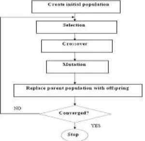
[image:2.612.376.526.539.685.2]

In many cases, the number of offspring‘s that an individual can except to produce in the next generation. This simple genetic procedure constantly produces even fitter offspring through successive generations. This process gradually leads the search towards a global optimum solution. A flowchart for a GA is shown in figure3.1

(3)

International Journal of Emerging Technology and Advanced Engineering

644 It involves nothing more than swapping of genes and string cloning. This allows GA to produce good results in circumstances which are hard to achieve through many conventional methods. The further attraction to such an algorithm is that it is extremely robust with respect to the complexity of the problem.

3.2 Phases in Genetic Algorithm

Typically, the genetic algorithms have three phases 1. Initialization

2. Evaluation 3. Genetic operation

 Initialization

Genetic Algorithms operate with a set of strings instead of a single string. This set of strings is known as a population and is put through the process of evolution to produce new individual strings. To start with, the initial population could be made up of chromosomes chosen at random or based on heuristically selected strings. The initial population should contain a wide variety of structures. The number of chromosomes in a population is usually selected to be between 30 and 100.We need two parents‘ population size and string length. Population size indicates the effective representation of whole search space in one population. It affects the efficiency and performance of GA. The selection of string length depends on the accuracy requirements of the optimization problem.

 Evaluation

In this phase, we determine the suitability of the solutions from the initial set of solution of the problem. For this suitability determination, we use a function called fitness function. This function is derived from the objective function and used in successive genetic operation.

For the minimization problem

f(x) = 1/(1+F(x)) (7)

Here f(x) is fitness function and F(x) is objective function.  Genetic Operation

In this phase we generate a new population from the previous population using genetic operators. They are

 Reproduction  Crossover  Mutation  Reproduction

This is the operator used to copy the old chromosome into matting pool according to its fittest valve. Higher the fitness of the chromosome more is number of the copies in the next generation chromosome. Chromosomes are selected from the population to be parents to crossover and produce offspring.

According to Darwin‘s fittest principle the best one should survive and create new offspring. That‘s why this operator is called selection operator. The commonly used reproduction operator is proportionate reproduction operator. The ith string in the population is selected with a probability proportional fi where f j is the fitness value for that string. The probability of selecting ith string is where ‗n‘ is the population size.

The various methods of selecting chromosomes for parents to crossover are;

 Roulette-wheel selection  Boltzmann selection  Tournament selection  Rank selection  Steady state selection

[image:3.612.390.534.368.529.2]

The commonly used reproduction operator is the roulette-wheel selection method where a string is selected from the mating pool with a probability proportional to the fitness.

Figure 2 A Roulette-wheel is marked for five individuals according to fitness value

The roulette-wheel mechanism is expected to make fi / fitavg copies of ith string of the mating pool. The average

fitness is

𝑓𝑖𝑡

_𝑎𝑣𝑔

=

𝑓𝑗 𝑛 𝑛

𝐽 =1 (8)

(4)

International Journal of Emerging Technology and Advanced Engineering

645 The best individual from the tournament is the one with the highest fitness which is the winner of individuals. Tournament competitor and the winner are then inserted into the mating pool. The tournament competition is repeated until the mating pool for generating new offspring is filled.

 Crossover

The basic operator for producing new chromosome is crossover. In this operator, information is exchanged among strings of matting pool to create new strings. The aim of the crossover operator is to search the parameter space. Crossover is a recombination operator, which proceeds in three steps. First, the reproduction operator selects at random a pair of two individual string for mating, then a crossover site is selected at random along the string length and the position values are swapped between two string following the cross site.

1. Single point crossover 2. Two point crossover 3. Multi point crossover 4. Uniform crossover 5. Matrix crossover

In the single point crossover, two individual strings are selected at random from the matting pool. Next, a crossover site is selected randomly along the string length and binary digits (alleles) are swapped between the two strings at crossover site. Suppose site 3 is selected at random. It means starting from the 4th bit and onwards, bits of strings will be swapped to produce offspring which is given in figure 3

Parent 1: x1 = {0 1 0 1 1 0 1 0 1 1 } Parent 2: x2= {1 0 0 0 0 1 1 1 0 0 } Offspring 1: x1= {0 1 0 0 0 1 1 1 0 0 } Offspring 2: x2= {1 0 0 1 1 0 1 0 1 1 } Figure 3 Single point crossover operations

In a two point crossover operator, two random sites are chosen and the contents bracketed by these sites are exchanged between two mated parents. If the cross site 1 is three and cross site 2 is six, the strings between three and six are exchanged which is shown in figure3.4. In a multipoint crossover, again there are two cases. One is even number of cross sites and other is odd no of sites. For even number of sites the string is treated as a ring and cross

Parent 1: x1= {0 1 0 1 1 0 1 0 1 1} Parent 2: x2= {1 0 0 0 0 1 1 1 0 0} Offspring 1: x1= {0 1 0 0 0 1 1 0 1 1} Offspring 2: x2= {1 0 0 1 1 0 1 1 0 0}

Figure 4 Two point crossover operation

Sites are selected around the circle uniformly at random if the number of cross sites is odd, then a different cross point is always assumed at the string beginning.

 Mutation

The final genetic operator in the algorithm is mutation. In general evolution, mutation is a random process where one allele of a gene is replaced by another to produce a new genetic structure. Mutation is an important operation, because newly created individuals have no new inheritance information and the number of alleles is constantly decreasing. This process results in the contraction of the population to one point, which is wished at the end of convergence process. Diversity is one goal of the learning algorithm to search always in regions not viewed before. Therefore, it is necessary to enlarge the information contained in the population. One way to achieve this goal is mutation. The role of mutation is often seen as providing a guarantee that the probability of searching any given string will never be zero and acting as safety net to recover good genetic material that may be lost through the action of selection and crossover. In GA‘s mutation is randomly applied with low probability in the range of 0.001 & 0.01 and modifies elements in the chromosome.

Here, binary mutation flips the value of the bit at the loci selected to be the mutation point. Given that mutation is applied uniformly to an entire population of strings, it is possible that a given string may be mutated at more than one point.

Offspring x1: 1 1 1 1 0 1 0 New offspring x2: 1 1 0 1 0 1 0

Figure 5 Mutation operation

IV. METHODOLOGIES

Here solution methodology which includes the encoding and decoding, constrained generation output are explained.

4.1 Encoding & Decoding

Decoding a binary string into unsigned integer can play very important role in GA implementation. The inequality power limit constraint is performed in such a way that the individual string is normalized over the unit‘s operating region. The inequality constraints are handled in the manner, which efficiently reduces the searching space, and thus enhances the performance of the system. Binary coded strings having 1‘s and 0‘s are used. The equivalent decimal integer of binary string is obtained as

(5)

International Journal of Emerging Technology and Advanced Engineering

646 Where, bij is the ith binary digit of the jth string and L is the number of strings or population size

V.FUZZY LOGIC CONTROLLED GENETIC ALGORITHM

This is mainly the hybrid system. Hybrid systems are those which employ integrated technologies to effectively solve problems. Hybrid systems are classified as sequential, auxiliary and embedded hybrids. Fuzzy-Genetic Hybrid system applicable on fuzzy optimization problems. The system obtains optimal solution to problems with fuzzy constraints and fuzzy variables. The hybrid systems have been demonstrated on the problems of optimization of structures (civil/machine tool) and obtain the optimal mix for high performance concrete. The optimal solution is obtained by Genetic Algorithm which crossover and mutation adjusted by fuzzy practical rules.

5.1 Fuzzy Rules for Crossover and Mutation Adjustment For better results and to get faster convergence, conventional GA modes have been modified. In recent years various techniques have been studied to achieve this objective, these include

 Using advanced string coding.

 Generating initial population with some prior knowledge.

 Establishing some better evaluation function.  Including new operators such as elitism, multi

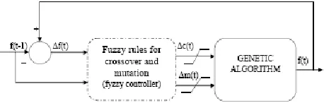
[image:5.612.61.290.538.611.2]

point or uniform crossover and creep mutation. FLCGA proposes a flexible Genetic Algorithm which based on fuzzy logic rules with the ability to adjust continuously the crossover and mutation parameters. Figure 6 presents the proposed block diagram of a fuzzy logic controlled genetic algorithm.

Figure 6 Global block diagram of the genetic parameters adjustment.

Crossover and Mutation are considered critical for GA convergence. A suitable value for mutation provides balance between global and local exploration abilities and consequently results in a reduction of the number of iterations required to locate the optimum solution.

Experimental results based in application of GA to any practical networks at normal and abnormal conditions with load incrementation indicated, that it is better to adjust dynamically the value of the two parameters, crossover and mutation. It is intuitive that for a small variation in the chromosomes in a particular population, the effect of crossover during this critical stage becomes insignificant therefore, creating diversity in the population is required by increasing mutation (High value) probability of the chromosome and reducing (Low value) the value of crossover, note that the terms, small and high are linguistic. The proposed approach employs practical rules interpreted in fuzzy logic rules to adjust dynamically the two parameters (crossover and mutation) during execution of the GA standard algorithm.

5. 2 Membership Function Design

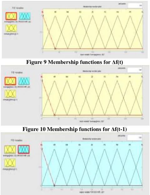
The variables chosen for this controller are change in average fitness (Δf(t)), change in average fitness in last iteration (Δf(t-1)), change in crossover probability (Δc(t)) and change in mutation probability (Δm(t)). In this, Δf(t) and Δf(t-1) are the input variables and Δc(t) is the crossover output and Δm(t) is the mutation output variable. The number of linguistic variables describing the fuzzy subsets of a variable varies according to the application. Usually an odd number is used. However, increasing the number of fuzzy subsets results in a corresponding increase in the number of rules. Each linguistic variable has its fuzzy membership function. The membership function maps the crisp values into fuzzy variables. The triangular membership functions are used to define the degree of membership. It is important to note that the degree of membership plays an important role in designing a fuzzy controller. Each of the input and output fuzzy variables is assigned nine linguistic fuzzy subsets varying from negative larger (NL) to positive larger (PL). Each subset is associated with a triangular membership function to form a set of nine membership functions for each fuzzy variable given in table 1.

NL NEGATIVE LARGER NR NEGATIVE LARGE NM NEGATIVE MEDIUM NS NEGATIVE SMALL ZE ZERO

PS POSITIVE SMALL

PM POSITIVE MEDIUM

PR POSITIVE LARGE PL POSITIVE LARGER

(6)

International Journal of Emerging Technology and Advanced Engineering

[image:6.612.53.313.135.236.2]

647 Figure 8 Block diagram of the fuzzy logic controller

[image:6.612.333.568.248.357.2]

The inputs to the crossover fuzzy logic controller are changes in fitness at two consecutive steps, i.e. Δf(t - l), Δf(t), and the output of which is change in crossover Δc(t). Membership functions of fuzzy input and output linguistic variables are shown in Figure 9,10,11. Δf(t-1), Δf(t) are normalized into the range of [-1.0, 1.0], and Δc(t) is normalized into the range of [-0.1, 0.1] according to their corresponding maximum values.

Figure 9 Membership functions for Δf(t)

Figure 10 Membership functions for Δf(t-1)

Figure 11 Membership functions for Δc(t)

The mutation operation is determined by the flip function with mutation probability rate, and the mutate bit is randomly performed. The mutation probability rate is automatically modified during the optimization process based on the fuzzy logic controller. The heuristic information for adjusting the mutation probability rate is if the change in average fitness is very small in consecutive generations, then the mutation probability rate should be increased until the average fitness begins to increase in consecutive generations.

Figure 12 Membership functions for Δm(t)

If the average fitness decreases the mutation probability rate should be decreased. only the change in output of mutation operator membership function which is shown in Figure 12.

The inputs to the mutation fuzzy controller are the same as those of the crossover fuzzy controller, and the output of which is the change in mutation Δm(t). The designs of the membership function for both input and rule base table for the fuzzy mutation controller is similar to these for the fuzzy crossover controller.

5.3 Fuzzy Rule Base for Solving The UCP

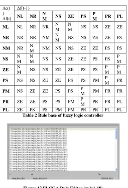
A set of rules which define the relation between the input and output of fuzzy controller can be found using the available knowledge in the area of designing UCP. These rules are defined using the linguistic variables. The two inputs, Δf(t) and Δf(t-1), result in 81 rules. The typical rules are having the following structure:

Rule 1: If Δf(t) is NL (negative larger) AND Δf(t-1) is NM (negative medium) then Δc(t) (output of fuzzy crossover) is NR (negative large).

Rule 2: If Δf(t) is PM (positive medium) AND Δf(t-1) is NL (negative larger) then Δc(t) (output of fuzzy crossover) is NS (negative small).

[image:6.612.55.295.368.680.2]

(7)

International Journal of Emerging Technology and Advanced Engineering

648 All the 81 rules governing the mechanism are explained in Table 1 where all the symbols are defined in the basic fuzzy logic terminology, it is shown in The Figure 13 &Figure 14.

Δc(t ) Δf(t)

Δf(t-1)

NL NR N

M NS ZE PS P

M PR PL NL NL NR NR N

M N

M NS NS ZE ZE

NR NR NR NM N

M NS NS ZE ZE PS

NM NR N

M NM NS NS ZE ZE PS PS

NS N

M N

M NS NS ZE ZE PS PS P M

ZE N

M NS NS ZE ZE PS PS P M

P M

PS NS NS ZE ZE PS PS PM P M PR

PM NS ZE ZE PS PS P

M PM PR PR

PR ZE ZE PS PS PM P

M PR PR PL PL ZE PS PS PM PM PR PR PL PL

[image:7.612.49.304.169.542.2]

Table 2 Rule base of fuzzy logic controller

Figure 13 FLCGA Rule Editor (rule1-19)

Figure 14 FLCGA Rule Editor (rule63-81)

5.4 Algorithm of FLCGA

The step-wise procedure is outlined below:

1. Read data, namely cost coefficients, ai, bi, ci, B-coefficients, Bij(i=1,2,….NG; J=1,2,….NG), step size and max allowed iterations, length of string, L, population size, pc probability of cross over, pm probability of mutations.

2. Generate all combinations (2N - 1). Check for the feasible combination corresponding to the satisfaction of the equality constraint (Generation ≥ Load demand) for each hour of the forecasted load.

3. Check that the Power output of each unit is within minimum and maximum generating limits of machines.

4. Set generation counter, k=0, fmax=0.0, and fmin=1.0

5. Increment the generation counter k=k+1 and set population counter j=0

6. Increment population counter j=j+16. Using gauss elimination method, find Pi

7. Find fitness if (fj > fmax) then set fmax = fj and if (fj<fmin) then set fmin=fj

8. If (j<L) then GOTO step 7 and repeat

9. Find population with max fitness and average fitness (fitavg)of the population

10. Select the parents for crossover using stochastic remainder roulette wheel selection method. 11. If the change in fitavg > 0, and keeps the same sign

in consecutive generations, Pc rate should be increased, otherwise Pc rate should be decreased. 12. Generate a random number (Rn), if Rn<Pc then

GOTO step 15 otherwise GOTO step 16

13. Perform single point crossover for the selected parents

14. If the change in fitavg is very small then Pm rate should be increased until the fitavg begins to increase. And if fitavg decreases the Pm rate should be decreased.

15. Generate a random number (Rn), if Rn<Pm, then GOTO step 18 otherwise GOTO step 19

16. Perform mutation operation for the selected parents

17. If (k<ITmax) then GOTO step 6 and repeat Satisfying the power balance equation.

18. Print the unit commitment schedule, operating fuel cost of each machine.

(8)

International Journal of Emerging Technology and Advanced Engineering

[image:8.612.130.223.155.253.2]

649 5.5 Flow Chart of FLCGA

Figure 15 Flow chart of FLCGA to solve UCP

5.6 Simulation Results

The results of UCP after the implementation on of proposed fuzzy logic controlled genetic algorithm are discussed. The algorithms are implemented in MATLAB to solve UCP problem. The main objective is to minimize the cost of generation of thermal plants using FLCGA. The performance is evaluated for two set generator data. Initial population and the probability values have been adjusted to settings for runs of a test method for a particular problem set. For the test method probability values have been adjusted through trial and error method, because of stochastic nature of GA, to bring out the best result that may be obtained from this method.

[image:8.612.324.578.315.614.2]

5.6.1Numerical results of test system four unit system: FLCGA Method.

Figure 16 Rule viewer of demand 520 MW the crossover 0.75

The power demand is considered to be 520MW. Crossover probability obtained is 0.75 for the above demand by using fuzzy logic.

5.6.2 Parameter setting of FLCGA for four unit systems

Length of the string, l = 16 Population of string, pop = 100 Crossover probability, pc = 0.75 Mutation probability, pm = 0.01

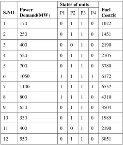
Based on the trails made, the best fitness value found to be converged at 48th generation out of 100 generations attempted shown in figure 17 for the demand of 520 MW. Convergence of Fitness value for the Demand of 700MW&1100MW also has shown in figure 18&19 respectively. Table 3 show the best results based on Unit Commitment Status and the Fuel Cost.

S.NO Power

Demand(MW)

States of units

Fuel Cost($) P1 P2 P3 P4

1 170 0 1 1 0 1022

2 250 0 1 1 0 1451

3 400 0 0 1 0 2190

4 520 0 1 1 0 2705

5 700 0 1 1 0 3780

6 1050 1 1 1 1 6172

7 1100 1 1 1 1 6552

8 800 1 1 1 0 4310

9 650 0 1 1 0 3504

10 330 0 1 1 0 1989

11 400 0 0 1 0 2190

12 550 0 1 1 0 3051

[image:8.612.62.289.475.625.2]

(9)

International Journal of Emerging Technology and Advanced Engineering

[image:9.612.67.284.120.250.2] [image:9.612.66.284.283.433.2]

650 Figure 17 Convergence of Fitness value for 520 MW

Figure 18 Convergence of Fitness value for 700 MW

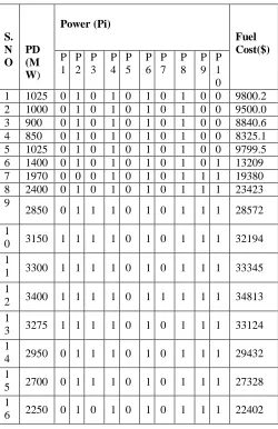
5.8 Numerical results of test system Ten unit system: FLCGA Method.

In order to test the efficiency of the GA to UCP, many benchmark tests have been carried out using data. Some of them are presented below.

Length of the string, l = 16 Population of string, pop = 200 Crossover probability, pc = 0.75 Mutation probability, pm = 0.01

[image:9.612.327.577.302.688.2]

Based on the trails made, the best fitness value found to be converged at 65th generation out of 200 generations attempted shown in figure 21 for the demand of 1025 MW

Table 4 Fuel cost for 10 unit systems with 24 hours

S. N O

PD (M W)

Power (Pi)

Fuel Cost($) P

1 P 2

P 3

P 4

P 5

P 6

P 7

P 8

P 9

P 1 0

1 1025 0 1 0 1 0 1 0 1 0 0 9800.2 2 1000 0 1 0 1 0 1 0 1 0 0 9500.0 3 900 0 1 0 1 0 1 0 1 0 0 8840.6 4 850 0 1 0 1 0 1 0 1 0 0 8325.1 5 1025 0 1 0 1 0 1 0 1 0 0 9799.5 6 1400 0 1 0 1 0 1 0 1 0 1 13209 7 1970 0 0 0 1 0 1 0 1 1 1 19380 8 2400 0 1 0 1 0 1 0 1 1 1 23423 9

2850 0 1 1 1 0 1 0 1 1 1 28572

1

0 3150 1 1 1 1 0 1 0 1 1 1 32194 1

1 3300 1 1 1 1 0 1 0 1 1 1 33345 1

2 3400 1 1 1 1 0 1 1 1 1 1 34813 1

3 3275 1 1 1 1 0 1 0 1 1 1 33124 1

4 2950 0 1 1 1 0 1 0 1 1 1 29432 1

5 2700 0 1 1 1 0 1 0 1 1 1 27328 1

[image:9.612.66.284.466.621.2]

(10)

International Journal of Emerging Technology and Advanced Engineering

651 1

7 2725 0 1 1 1 0 1 0 1 1 1 27547 1

8 3200 1 1 1 1 0 1 0 1 1 1 32745 1

9 3300 1 1 1 1 0 1 0 1 1 1 33345 2

0 3900 1 1 1 1 0 1 1 1 1 1 36037 2

1 2125 0 1 0 1 0 1 0 1 1 1 21332 2

2 1650 0 1 0 1 0 1 0 1 1 1 16856 2

3 1300 0 1 0 1 0 1 0 1 0 1 12522 2

4 1150 0 1 0 1 0 1 0 1 0 1 11967

[image:10.612.337.561.102.243.2]

5.9 Summary

In this chapter fuzzy logic controlled genetic algorithm were discussed. These formulations were applied to UCP, by varying the crossover probability and mutation probability during the GA method. The Standard data‘s of test systems were analyzed through the simulation in MATLAB environment.

VI. C

ONCLUSION

[image:10.612.343.559.289.433.2]

(11)

International Journal of Emerging Technology and Advanced Engineering

652

R

EFERENCES

[1] Wood A. J. and Woolenberg B. F., ―Power generation, operation and control‖, New York, NY: John Wiley Sons; 1996.

[2] Gerald B. Sheble and George N. Fahd, ―Unit Commitment Literature Synopsis.‖ IEEE Trans. Power System, Vol. 9, No. 1, February1994.

[3] N. P. Pandhy, ―Unit Commitment-A Biological Survey.‖ IEEE Trans. Power Systems, Vol. 19, No. 2, May 2004.

[4] N. P. Pandhy, ―Unit Commitment using Hybrid models: A Comparative Study for Dynamic Programming, Expert System, Fuzzy System and Genetic Algorithm.‖ Electric Power and Energy Systems 23 (2000) 827-836, February 1994.

[5] M. Dorigo, and Thomas Stuzle, ―An Experimental Study of the Simple Ant Colony Optimization Algorithm.‖ Proceedings of 2001 WSES International Conference on Evolutionary Computation (EC‘01), N. Mastorakis (Ed.), WSES-Press International, 253 – 258.

[6] Sishaj P. Simon, N. P. Pandhy and R. S. Anand ―A new Ant Colony System approach to Unit Commitment Problem.‖ Proceeding of National Power System Conference, NPSC 2004, IIT Madras, India, and December 2004. pp. 1061 – 1066.

[7]Javad Ebrahimi, Seyed Hossein Hosseinian, and Gevorg B. Gharehpetian,“Unit Commitment Problem Solution Using Shuffled Frog Leaping Algorithm‖ IEEE Transactions on Power Systems, Vol. 26, No. 2, May 2011 [8]C.Y.Chung,Han Yu, and Kit Po Wong, ―An Advanced Quantum-Inspired Evolutionary Algorithm for Unit Commitment‖ IEEE Transactions on Power Systems, Vol. 26,No.2,May2011

[9]Moosa Moghimi Hadji, and Behrooz Vahidi, ―A Solution to the Unit Commitment Problem Using Imperialistic Competition Algorithm” IEEE Transactions on Power Systems, Vol. 27,No.1, February 2012

[10]Irina Ciornei,and Elias Kyriakides, ―Hybrid Ant Colony-Genetic Algorithm (GAAPI) for Global Continuous Optimization‖ IEEE Transactions On Systems, Man, And Cybernetics—PART B: Cybernetics, Vol. 42, No. 1, February 2012

[11] Arroyo M. C. and Jose M., ―A computationally efficient mixed-integer linear formulation for the thermal unit commitment problem‖, IEEE Transactions on Power System, Vol. 21, No. 3, pp. 1371-348, 2006.

[12] Arroyo J. M. and Conejo A. J., ―A parallel repair genetic algorithm to solve the unit commitment problem‖, IEEE Transactions on Power System, Vol. 17, No. 4, pp. 1216-1224, 2002.

[13] Cheng C. P., Liu C.W. and Liu C. C., ―Unit commitment by Lagrangian relaxation and genetic algorithm‖, IEEE Transactions on Power System, Vol. 15, No. 2, pp. 707-714, 2000.

[14] Sisworahardjo.N.S., and El-Keib.A.A., ―unit commitment using the ant colony search algorithm‖, Proceedings of the 2002 Large Engineering Systems Conference on Power Engineer, 2002 IEEE, 0-7803-7520-3.

[15] T. O. Ting, Student Member, IEEE, M. V. C. Rao, and C. K. Loo, Member, IEEE ―A Novel Approach for Unit Commitment Problem via an Effective Hybrid Particle Swarm Optimization‖ IEEE transactions on Power Systems, vol. 21, no. 1, february 2006,411-418