From a profiled diffuser to an optimized absorber

From a profiled diffuser to an optimized 

absorber

Wu, T, Cox, TJ and Lam, YW

http://dx.doi.org/10.1121/1.429596

Title

From a profiled diffuser to an optimized absorber

Authors

Wu, T, Cox, TJ and Lam, YW

Type

Article

URL

This version is available at: http://usir.salford.ac.uk/14652/

Published Date

2000

USIR is a digital collection of the research output of the University of Salford. Where copyright 

permits, full text material held in the repository is made freely available online and can be read, 

downloaded and copied for non­commercial private study or research purposes. Please check the 

manuscript for any further copyright restrictions.

From a profiled diffuser to an optimized absorber

T. Wu, T. J. Cox, and Y. W. Lam

School of Acoustics and Electronic Engineering, University of Salford, Salford M5 4WT, United Kingdom

共Received 28 October 1999; revised 24 March 2000; accepted 23 April 2000兲

The quadratic residue diffuser was originally designed for enhanced scattering. Subsequently, however, it has been found that these diffusers can also be designed to produce exceptional absorption. This paper looks into the absorption mechanism of the one-dimensional quadratic residue diffuser. A theory for enhanced absorption is presented. Corresponding experiments have also been done to verify the theory. The usefulness of a resistive layer at the well openings has been verified. A numerical optimization was performed to obtain a better depth sequence. The results clearly show that by arranging the depths of the wells properly in one period, the absorption is considerably better than that of a quadratic residue diffuser. © 2000 Acoustical Society of

America. 关S0001-4966共00兲01308-4兴

PACS numbers: 43.55.Ev, 43.55.Dt关JDQ兴

INTRODUCTION

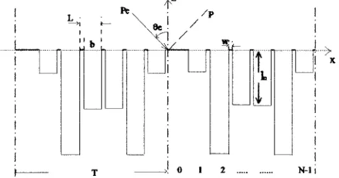
Profiled diffusers were invented by Schroeder1 in the 1970s. An example of the one-dimensional Schroeder diffus-ers is shown in Fig. 1. They are periodic surface structures with rigid construction; the elements of the structure are wells of the same width separated by thin fins. Within one period, the depths of the elements vary according to a pseudo-stochastic sequence.

The basis behind the Schroeder diffuser is as follows: When the sound is incident on the surface of the structure, plane waves travel down and up each wells. The returning waves at the entrances of the wells no longer have the same phases because of the different depths they have traveled. If the phase differences are appropriate, the diffuser will dis-perse the sound rather than specularly reflect it, and thus generate diffusion in the far field. For this purpose, Schroeder exploited the Fourier transform of the surface re-flection factors to choose the depth sequence in one period, as it approximately gives the far field diffracted pressure dis-tribution. The most popular Schroeder diffuser is the qua-dratic residue diffuser共QRD兲, which employs the quadratic residue sequence to determine the well depth. The Fourier transform of the QRD surface reflection factors gives a con-stant power spectrum leading to even energy diffraction lobes. The QRD has been widely used in concert halls, the-atres, and studio monitor rooms.2,3

The QRD was designed to diffuse rather than absorb sound, although for some time there was anecdotal evidence of absorption. Dramatic levels of absorption from Schroeder diffusers were measured by Fujiwara and Miyajima4in 1992. They reported the unexpectedly high measured absorption of a poorly constructed QRD at low frequency, which they could not explain. It was later found5 that the quality of construction was to blame for some of the excess absorption. Kuttruff6tried to explain the absorption by assuming that the total sound pressure on the diffuser plane was constant. This led to an absorption based on the same average surface ad-mittance, which generated additional possible air flow be-tween adjacent wells. This additional air flow was associated with the excess absorption of the diffusers, but this air flow

is not explicitly included in the average admittance model. He could only find agreement with Fujiwara’s data when he reduced the width of the wells to an unrealistic one-tenth of the width in the real diffuser. Mechel thoroughly investigated the Schroeder diffuser in his paper in Acustica7 and in greater detail in his book.8He described the absorption effect for the near field as well as the directivity for the far field analysis, with and without viscous and thermal losses in and in front of the wells using a Fourier wave decomposition model. Mechel demonstrated that resistive layers at the well entrances turn these diffuser structures into potentially useful and practical absorbers. Furthermore, he discussed how us-ing a primitive root sequence to determine the well depths of the structure could result in a better absorber than the more common quadratic residue sequence. Unfortunately, there were no corresponding experimental results to verify the findings, something which is added later in this paper.

In this paper, the sound absorption by the one-dimensional Schroeder diffuser is studied both theoretically and experimentally. The Schroeder structure can be used to make an effective absorber or a low loss diffuser depending on the geometry and construction of the device. Since ab-sorption is more of a concern here than diffusion, the width of the wells has been reduced for this study compared to QRDs designed for diffusive purposes. The losses in the wells caused by the viscous and thermal conduction have been considered. To predict the surface sound absorption, the method used by Mechel is used. The use of a resistive layer on the surface to improve the absorption of the structure is investigated in some detail.

As shall be shown later, a optimum diffuser does not necessary produce the best absorption. It is possible to pro-duce a configuration that is a better absorber than those based on the quadratic residue sequence. This is done by producing many well-tuned and well-distributed resonance frequencies by choosing the depth sequence in one period using an optimization approach.

I. PREDICTION METHOD

surface admittance, another uses Fourier analysis. The former was introduced by Kuttruff by assuming uniform pressure on the entrance of the structure. In many cases, however, as he indicated, it is only an approximate method, as it does not properly model the mutual interference be-tween the differently tuned wells caused by different depths in one period. The later method, i.e., Fourier analysis, more correctly considers the coupling between the wells, and thus is more rigorous. In this paper only Fourier analysis method will be discussed and used in the predictions. Figure 1 shows a sketch of a one-dimensional QRD structure, together with the coordinate system. The expression of the depth sequence,

ln, in one period of a one-dimensional QRD is well known

1

as

ln⫽

c mod共n2,N兲

N共2 fr兲

, n⫽0,1,...,N⫺1. 共1兲

where fris the design frequency, N is the prime number, and

c is the speed of sound in air. As shown in Fig. 1, the diffuser

is periodic with N wells in one period. The period is T

⫽N*L wide with the grid length of one well, L⫽b⫹w,

where b is the well width and w is the wall thickness be-tween the wells.

A. Energy losses in the wells

Normally the well width of the QRD is quite large to minimize absorption. However, in this study, the width of the wells needs to be reduced to get higher absorption. In this case, the losses caused by the viscous and thermal conduc-tion in the narrow wells cannot be neglected. In general, in the middle frequency range of interest, the width of the wells

b is usually quite narrow compared with the incident

wave-length, i.e., bⰆ␭/2, so that there is only fundamental mode propagating in each well.

When describing the sound propagation in a narrow slit, three waves will be of concern: propagating wave, thermal wave, and shear wave. In many cases of practical interest, the attenuation caused by the thermal wave and viscous wave only occurs in the boundary layers, which are of a fraction of a millimeter thick. Usually their effects can be incorporated into the boundary conditions on the propagating wave. Morse and Ingard9 derived the complex wave number in a cylindrical tube. The method can also be used for a narrow slit.

Assuming that the slit has two infinite parallel rigid walls, then it is somewhat more convenient to run the z axis along the central line of the slit. Because the boundary sur-face is rigid, the particle velocity u and the temperature fluc-tuation ␶at the surface are zero. The propagation wave for fundamental mode has acoustic pressure pp, temperature

␶p, and normal upxand tangential upz velocity:

9,10

pp⫽cos

冉

␲qx b

冊

e

⫺jk_tz_ej␻t_,

␶p⫽

␥⫺1

␣␥ cos

冉

␲qx

b

冊

e

⫺jk_tz_ej␻t_,

共2兲

upx⫽

1

j␻␳

␲q b sin

冉

␲q兩x兩 b

冊

e

⫺jk_tz_ej␻t_,

upz⫽

kt

␳ckcos

冉

␲qx b

冊

e

⫺jk_tz_ej␻t_,

where k_t2⫽k2_⫺(␲q/b)2_{, k⫽␻/c is the wave number,␳ is} the air density, and␥⫽(C_P/C_V) is the ratio of the specific heat,⬇7/5 for air. The constant q can be adjusted to fit the boundary conditions by incorporating the thermal wave and shear wave in the boundary layers. Following the method used by the Morse and Ingard,9for width bⰇd_v,dh, where

d_v,dh are the thickness of the viscous and thermal boundary

layers, q can be defined for a narrow slit:

共␲q兲2⫽⫺共1⫺j兲k2b关d_v⫹共␥⫺1兲dh兴. 共3兲

This gives the propagation number as

kt⫽

冑

k2⫺

冉

␲q b

冊

2

⬇k⫹ k

2b共1⫺j兲关dv⫹共␥⫺1兲dh兴 共4兲 for air at atmospheric pressure and room temperature, d_v,dh

can be determined10as

d_v⫽

冑

2␮

␳␻⬇0.21

1

冑

f, dh⫽

冑

2K

␳␻C_p⬇0.25

1

冑

f 共cm兲, 共5兲

where f is sound frequency, and ␮, K, and Cp are the

prop-erties of gas. ␮is the coefficient of viscosity, K is the ther-mal conductivity, and Cpis the heat capacity per unit mass at

constant pressure.

Once the sound propagation in the slit is known, the inward impedance on the surface of well with length ln can

be easily derived as

Z共l_n兲⫽⫺j␳_eck kt

cot共k_tl_n兲, 共6兲

where␳_eis the effective density of air in the slit:11

␳e⫽␳关1⫹共1⫺j兲dv/b兴 共7兲

so that the inward normalized specific impedance of the well with length ln is then

␨共ln兲⫽

Z共ln兲

␳c

⫽⫺j兵1⫹共1⫺j兲关dv⫺共␥⫺1兲dh兴/2b其cot共ktln兲.

[image:3.612.58.297.37.163.2]

共8兲 FIG. 1. One-dimensional quadratic residue diffuser for N⫽7, 2 periods

shown.

B. Prediction of absorption by QRD

[image:4.612.315.561.51.180.2]

The analysis below closely follows the method used by Mechel.7 The sound field in front of the diffuser, shown in Fig. 1, is decomposed into the incident plane wave p_e(x,z) and scattered field ps(x,z), which is made up of propagating

and nonpropagating evanescent waves:

p共x,z兲⫽pe共x,z兲⫹ps共x,z兲, 共9兲

pe共x,z兲⫽Pe•ej共⫺xkx⫹zkz兲,

where kx⫽k sin␪e, kz⫽k cos␪e, 共10兲

ps共x,z兲⫽

兺

n⫽⫺⬁

⫹⬁

Anej共⫺x␤n⫺z␥n兲. 共11兲

Since the QRD is periodic, the scattered field is also periodic in x. Therefore the wave numbers in the x and z directions of the spatial harmonics are 共the first from the periodicity, the latter from the wave equation兲

␤n⫽kx⫹n

2␲

T ;

共12兲

␥n

2_⫽k2_⫺␤

n

2_⇒␥

n⫽⫺j k

冑

冉

sin␽e⫹n

␭ T

冊

2

⫺1,

where␭⫽2␲/k is the wavelength. The corresponding radi-ating harmonics indices ns, which can propagate to the far

field, are determined from

冉

sin␪e⫹ns

␭ T

冊

2

⭐1. 共13兲

Considering the outward particle velocity along the posi-tive z direction, the relation of pressure and particle velocity on the surface is ␳cvz(x,0)⫽⫺G(x) p(x,0). This gives

cos␪ePe⫺

兺

n⫽⫺⬁

⫹⬁ _␥

n

k Ane

⫺jxn2␲/T

⫽G共x兲

冋

Pe⫹

兺

n⫽⫺⬁

⬁

Ane⫺jxn2␲/T

册

. 共14兲

Since G(x) is periodic with a period T, we apply a Fourier analysis:

G共x兲⫽

兺

n_⫽⫺⬁

⫹⬁

gne⫺jn(2␲/T)x,

共15兲

gn⫽

1

T

冕

0

T

G共x兲e⫹jn(2␲/T)xdx.

Equation 共15兲 inserted into the boundary condition gives, after multiplication by ejm(2␲/T)x and integration over T:

兺

n⫽⫺⬁

⫹⬁

An

冉

gm⫺n⫹␦m,n

冉

␥n

k

冊冊

⫽Pe共␦m,0cos␪e⫺gm兲; m⫽⫺⬁,...,⫹⬁, 共16兲 where

␦m,n⫽

再

1, m⫽n

0, m⫽n,

and the infinite large system of equations will be terminated at the index limits n,m⫽⫾2*N, where N is the number of

wells in one period. By solving the above equations, the coefficients A_n can be obtained.

The absorption coefficient of diffuser is then

␣共␪e兲⫽1⫺

冏

A0

Pe

冏

2

⫺ 1

cos␪e n

兺

_s⫽0

冏

An_s

Pe

冏

2

冑

1⫺共sin␪e⫹ns␭/T兲2;

共17兲 the summation runs over radiating spatial harmonics only. Evidently the second term is the specular reflection, and the third term is due to scattering.

If a resistive layer is applied on the surface of structure to enhance the absorption, the only replacement made in the above method is G(x)→1/(R⫹␨well), where R is the nor-malized effective impedance of the resistive layer, and ␨well is the input normalized impedance of a well.

II. EXPERIMENTAL AND THEORETICAL RESULTS

A. Methods of measurement

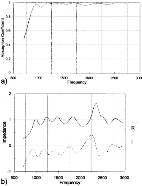
Two types of samples, one with constant length slits and the other a one-dimensional QRD, were built from a square tube that had a cross-section size 54 mm⫻54 mm. Because of tube’s size, the QRD are limited to: prime number 7, design frequency f r⫽980 Hz, the maximum length of wells 10 cm, well width b⫽6 mm, and separation wall thickness

w⫽1 mm. The length sequence has been listed in Table I, as ‘‘QRD.’’ The wells were terminated by MDF共Medium Den-sity Fiberboard兲 which has been varnished three times. The wells are separated by aluminum sheets. In order to compare fairly, the corresponding constant length structure is com-posed of seven slits with the same width as the QRD and with all the wells having a length of 10 cm. The whole sample is sealed with petroleum jelly as good as possible.

A method similar to the standard two microphone method12 is used to measure the surface impedance of the sample in the impedance tube. Consequently, the results pre-sented here are restricted to normal incidence. Furthermore, the normal incidence absorption coefficient is computed for the impedance from the well-known formula:13

TABLE I. Depth sequences of different structures共in cm兲.

QRD Random sequence Optimization Without mirror-image With mirror-imagea

1 2 1 2

0.0 0.0 3.6 2.5 10.0 4.8 2.5 1.0 10.0 10.0 9.2 3.4 10.0 3.0 5.6 3.8 8.5 3.7 5.0 5.0 9.1 9.4 7.2 8.6 5.0 7.0 6.7 5.9 5.8 5.7 10.0 9.0 8.2 7.3 3.9 8.3 2.5 10.0 4.5 4.8 4.3 10.0

a

[image:4.612.67.293.114.207.2]

␣⫽_关1⫹Re共4 Re_␨兲兴2共_⫹␨兲_{关Im共␨兲兴}2, 共18兲 where Re(␨) and Im(␨) are the real part and imaginary part of the normalized impedance, respectively.

The effect of the resistive layers is also tested. A thin wire mesh with resistance 550 rayl 共MKS兲, whose normal-ized specific acoustic impedance is 1.325, is applied in front of the sample.

B. Theoretical prediction

To predict the experimental results, there are a few things that should be noted:

First, because the sample is set up in the impedance tube with rigid walls, the prediction in Sec. I B cannot be used directly. The period must be doubled to take into account the mirror imaging effect of the side walls. For example, consid-ering the tested QRD with N⫽7, the depth sequence in one period is 0 1 4 2 2 4 1. An image sequence 1 4 2 2 4 1 0 will be created by the rigid walls. So, in fact, this system has 14 elements in one period.

Second, when predicting the absorption coefficient of the sample with wire mesh, the mass effect of the wire mesh has to be considered. In most cases, wire mesh can be treated as rigid. But a thin wire mesh is flexible, and there will be an inertial mass contribution resulting from the induced motion of the sheet.14So the normalized effective impedance of the wire mesh is

R⫽

冋

Rm共␻m兲

2

R_m2⫹共␻m兲2⫹j

R_m2共␻m兲

R_m2共␻m兲2

册

冒

␳c, 共19兲

where Rm and m are, respectively, the resistance and mass

per unit area of wire mesh.

C. Results and discussions

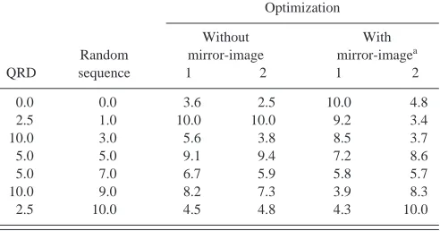
For conciseness, the following abbreviations in the nor-malized impedance graphs will be adopted throughout this paper. The real part of normalized impedance will be R, and the imaginary part I.

Figures 2 and 3 show the predicted and measured sound absorption coefficient for the constant slits and QRD without wire mesh, and Figs. 4 and 5 show the results with wire mesh. The agreement is good, especially for the results with

wire mesh. Without wire mesh, the absorptions are small and very difficult to measure, especially for the constant slits in Fig. 2. Figure 3 contains two important features. First, around the second peak, the absorptions are higher than pre-diction, it may due to both the gaps in the QRD structure and the resonant vibration of the aluminum sheet, which sepa-rated the wells; Second, there is a very sharp absorption peak around 2330 Hz. This only appears in the prediction if the mirror imaging of the rigid walls is modeled. It would not appear for a straight periodic QRD. Comparing Figs. 2 and 3, it is clear that the absorption of the QRD is much higher than the corresponding constant slits. In Figs. 4 and 5, it can be seen that the resonant frequencies are slightly shifted down when the wire mesh is added. This is due to the mass effect introduced by the thin flexible wire mesh. Comparing the absorption in Figs. 4 and 5, higher and more uniform absorp-tion is found for the QRD compared with the constant slit surface.

III. ABSORPTION MECHANISM DISCUSSION

[image:5.612.318.558.33.184.2]

Comparing the absorption of the constant length struc-ture in Fig. 2 and the absorption of the QRD in Fig. 3, al-though less cells of the QRD are resonating at a particular frequency, it generates higher absorption than the constant slits, even at the resonance frequencies of constant slits, where all slits contribute. This is because the variable depths of the wells create a nonuniform surface impedance that scat-ters the incident sound. The scattering enhances the propa-FIG. 2. Absorption coefficient of constant length slit sample.

[image:5.612.56.295.34.174.2]

FIG. 3. Comparison between the prediction and experiment for the QRD.

FIG. 4. Absorption coefficient from constant slit sample with 550 Rayls wire mesh on the entrance of the slit.

[image:5.612.319.559.575.713.2]

gation of the sound wave between wells and hence increases the sound absorption. The impedance graphs of them are typical for pipe systems, except that the QRD has nonuni-form resonant frequencies caused by depth variety and slightly higher resistance than constant slits because of the coupling of wells. Applying facing wire-mesh can improve the absorption coefficient significantly across the whole fre-quency range. Figure 6 shows the normalized specific acous-tic impedance corresponding to the constant slits tested in Fig. 4, with a wire mesh glued on the opening of slits, and Fig. 7 shows that corresponding to the QRD tested in Fig. 5 with glued facing wire mesh. For constant length slits, ap-plying wire mesh shifts down the resonance frequencies共the fundamental and first harmonic兲because of the mass effect. The real part remains close to the resistance of the wire mesh at 1.325. There is no coupling between the wells that may effect the impedance of whole structure. The absorption is high at the resonance frequencies, but elsewhere is poor. For the QRD, Fig. 7 shows that applying the wire mesh not only shifts down the resonance frequencies, it also smooths the imaginary part and real part of impedance. The imaginary part stays close to zero. This is the reason why high absorp-tion is achieved across the whole frequency range. However, the resistive part is also substantially increased away from unity, leading to a slightly smaller absorption coefficient at resonances. This indicates that the choice of wire mesh is important in optimizing the absorption.

IV. OPTIMIZATION

As mentioned before, the depth sequence of a Schroeder diffuser is very important to the absorption of whole struc-ture. In this section, a numerical optimization method,15 downhill simplex method, is used to tune this sequence. By optimizing the sequence, many tuned and well-distributed resonance frequencies can be generated, and higher absorption can be achieved.

A. Optimization process and ‘‘absorption parameter’’ discussion

The process to produce an optimum profiled absorber is based on an iterative process:

共1兲 An absorber with N wells in one period is constructed with a randomly determined depth sequence.

共2兲 Absorption coefficients of the absorber is calculated by the Fourier analysis method across the frequency range of interest.

共3兲A single figure cost function is calculated which can mea-sure the degree of broadband absorption.

共4兲 The well depths are altered according to the Downhill Simplex method.

共5兲 Steps 共2兲–共4兲 are repeated until a minimum in the cost function is found indicating an optimum absorber.

There are two cost functions which have been used in the optimization: one is ⫺兺i_⫽1

N _␣

i/N, where ␣i is absorption

coefficient, N is the number of frequencies chosen in the frequency range interested, and the other is

冑

(兺i_⫽1

N

Xi

2 )/N, where Xi is the imaginary part of specific acoustic

imped-ance. The first parameter measures the negative of the mean absorption, hence the minimum value gives the highest av-erage absorption. The second one is used because absorption is strongly related to the impedance on the surface of the structure. When the imaginary part of the impedance stays close to zero, high absorption is usually obtained. But one thing that should be noticed here is that the coupling between the wells may cause real part of the impedance to increase and result in less absorption. It is necessary to run the opti-mization process many times with different starting condi-tions. The reason for this is that the minimization is being carried out within bounded space. The space hold many local minima within which the minimization routines could be-FIG. 5. Comparison between predicted and measured absorption for the

[image:6.612.54.297.33.178.2]

QRD with facing wire mesh 550 Rayls.

FIG. 6. Normalized specific impedance corresponding to Fig. 4.

[image:6.612.320.557.34.197.2] [image:6.612.57.296.583.723.2]

come trapped, particularly at the edges. The results shown below are the best results from many attempts of the iteration process. This does not exclude the possibility that from some particular starting point yet untried there might have a better minimum available.

B. Optimization examples: Theoretical results

As an example, the QRD with the same parameters as that tested in Fig. 3 has been optimized for normal plane wave incidence. In order to compare the results fairly, the maximum lengths of the wells are restricted to 10 cm in the optimization program. The first ‘‘absorption parameter’’ cost function, based on the mean absorption coefficient, is used. The frequency range for the optimization is 700 Hz–3000 Hz. The obtained depth sequence of optimized surface struc-tures without and with wire mesh have been listed in Table I as ‘‘Optimization-Without mirror-image’’ 1 and 2, respec-tively.

The results of the comparison with optimized structure, QRD and structure employing random depth sequence, with-out facing wire mesh on the structure, is illustrated in Fig. 8. The random depth sequence is listed in Table I under ‘‘ran-dom sequence.’’ It clearly shows that the optimized structure improves the absorption coefficient significantly compared with other two. Its mean absorption coefficient is increased from 0.16 to 0.35 compared with the QRD. In the QRD, the zero depth well does not contribute directly to the absorption as there are no viscous losses due to progragation in this well, so its removal is useful. As there were more nonuni-form depths in one period of the optimized structure than the original QRD, more resonance frequencies are generated within the whole frequency range, and the real part of the optimized surface impedance is also improved because of the better coupling of wells when compared to the QRD and random depth sequence. But as shown in Fig. 8, the absorp-tion coefficient is not smooth with many peaks and troughs according to the resonance and anti-resonance frequencies, which is inevitable because of the small resistive part.

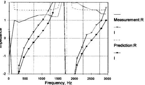
The result of the optimization with a facing wire mesh is shown in Fig. 9. This wire mesh has a small flow resistance 55 rayls共MKS兲, which is a normalized specific impedance of 0.1325. Figure 9共a兲 shows that the optimized structure is

obvious a good absorber, with a mean absorption coefficient of 0.96. And Fig. 9共b兲shows that, not only does the imagi-nary part stay close to zero, but the real part of the specific impedance had been raised close to unity. This is more than the flow resistance of the wire mesh can achieve alone. This example demonstrates that optimized the depth sequence can improve the absorption of structure significantly, and down-hill simplex method is fast and efficient for this purpose.

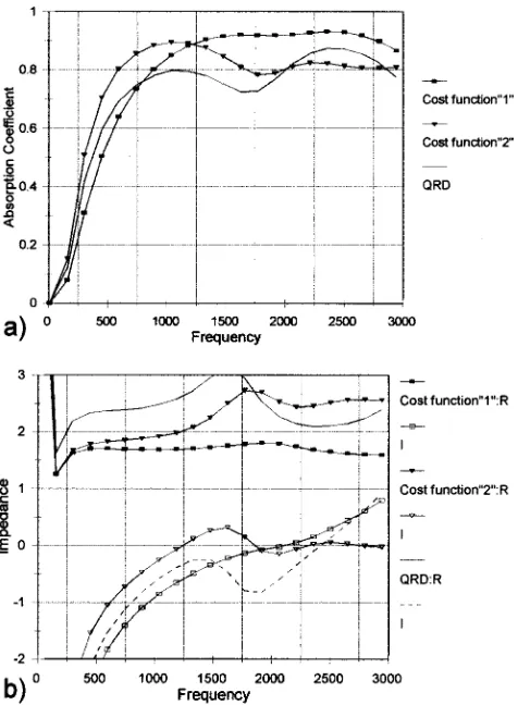
As mentioned before, there are two cost functions that can be used to measure the absorption, the following discus-sion is about the difference in results obtained by using them separately. The base structure is the same as above, but the facing flow resistance is now at 550 rayl共MKS兲, which is ten times as used before. The results are shown in Fig. 10.

[image:7.612.317.555.33.344.2]

Regarding Fig. 10共a兲, it is hard to say which cost func-tion is better. The first cost funcfunc-tion parameter, average ab-sorption, generated a high absorption across the frequency range; but the second cost function parameter, minimum imaginary Z, produces higher absorption at low frequency. Figure 10共b兲also shows other important points. The second, impedance based ‘‘cost function,’’ which is intended to pro-duce the imaginary part close to zero, does work. But it also pushes the real part higher at some frequencies at the same time, this induces less absorption at these frequencies; The first, absorption based ‘‘cost function,’’ seems to optimize the real part and keep it close to 1, and therefore achieving the higher absorption. Although the imaginary part of imped-ance is not as close to zero as in the other case, there is no doubt it is optimized as well. Therefore, for the facing sheet FIG. 8. Comparison of the absorption coefficient for the optimized surface,

the QRD, and random sequence structure.

FIG. 9. Optimized structure with facing wire-mesh flow resistance 55 Rayls.

共a兲absorption coefficient;共b兲normalized specific impedance.

[image:7.612.55.296.33.182.2]

that has higher resistance, it is better to use the imaginary part cost function in the optimization process, where the real part cannot be reduced. On the other hand, the first cost function is better, for the lower facing resistance.

C. Experimental verification

Again the tests carried out in the impedance tube, and the optimizations had to be repeated with and without wire mesh to take into account of the mirror imaging effect of the impedance tube samples. The resistance of the wire mesh is Rayls 共MKS兲, which is a normalized specific impedance of 0.434. The optimized structures used in the experiments have

depth sequences shown in Table I, labeled as ‘‘Optimization-with mirror-image’’ 1 and 2, where ‘‘1’’ represents a depth sequence without wire mesh and ‘‘2’’ with wire mesh. The structures are built according to the above depth sequence, and other parameters are the same as tested before: seven wells, b⫽6 mm, w⫽1 mm.

Figure 11 is the comparison between the prediction and experiment absorption data without wire mesh, it shows that in generally they match each other. But there are two peaks which are not expected. It is suggested that they may be caused by the resonant vibration of the aluminum sheets, or higher modes generated in the wells.16 Figure 12 shows the tested result of the optimized structure with wire mesh; the very good agreement can be clearly seen. The improvement compared with the QRD and random depth sequence struc-ture is also illustrated.

V. CONCLUSIONS

The above study has shown that the variable depth se-quence concept can be used to significantly improve the ab-sorption and impedance characteristics of conventional con-stant depth design. A theory for the prediction of the enhanced absorption was presented and verified by normal incidence measurements on a variety of samples, with and without facing wire meshes. The prediction generally agrees well with experiments and the accuracy is particularly good in cases where a wire mesh is present. An optimization al-gorithm has been implemented. It was used to demonstrate the improvements in normal incidence absorption perfor-mance that can be achieved by optimizing the depth se-quence. The optimized structure was tested in impedance tube measurements. The data generally agree with the pre-dicted performance. Further work will be needed to extend the investigation to 2D and to test the optimised samples for the oblique incident sound.

ACKNOWLEDGMENTS

[image:8.612.57.295.31.355.2]

This work was funded by Engineering and Physical Sci-ences Research Council 共EPSRC兲 of Britain, under Grant No. GR/L34396.

FIG. 10. Comparison of the results using different ‘‘absorption cost func-tions.’’共a兲absorption coefficient;共b兲normalized specific impedance.

[image:8.612.316.558.33.183.2]

FIG. 11. Comparison of the predicted and measured absorption coefficient for optimized surface.

[image:8.612.55.297.572.712.2]

1_{M. R. Schroeder, ‘‘Binaural dissimilarity and optimum ceilings for} con-cert halls: More lateral sound diffusion,’’ J. Acoust. Soc. Am. 65, 958– 963共1979兲.

2

P D’Antonio and T. J. Cox, ‘‘Two decades of room diffusers. Part 1: Applications and design,’’ J. Audio. Eng. Soc. 46, 955–976共1998兲. 3_{P D’Antonio and T. J. Cox, ‘‘Two decades of room diffusers. Part 2:}

Measurement, prediction and characterisation,’’ J. Audio. Eng. Soc. 46, 1075–1091共1998兲.

4

K. Fujiwara and T. Miyajima, ‘‘Absorption characteristics of a practically constructed Schroeder diffuser of quadratic-residue type,’’ Appl. Acoust.

35, 149–152共1992兲.

5_{K. Fujiwara and T. Miyajima, ‘‘A study of the sound absorption of a} quadratic-residue type diffuser,’’ Acustica 81, 370–378共1995兲. 6_{H. Kuttruff, ‘‘Sound absorption by pseudostochastic diffusers共Schroeder}

diffusers兲,’’ Appl. Acoust. 42, 215–231共1994兲.

7_{F. P. Mechel, ‘‘The wide-angle diffuser—A wide-angle absorber?,’’} Acustica 81, 379–401共1995兲.

8

F. P. Mechel, Schallabsorber共S. Hirzel Verlag, Stuttgart, 1998兲, Vol. III, Chap. 5.

9_{P. M. Morse and K. Ingard, Theoretical Acoustics共McGraw-Hill, New}

York, 1968兲, Chap. 9, pp. 519–522.

10_{P. M. Morse and K. Ingard, Theoretical Acoustics共McGraw-Hill, New}

York, 1968兲, Chap. 6, pp. 285–291.

11_{J. F. Allard, Propagation of Sound in Porous Media: Modeling Sound}

Absorbing Materials 共Elsevier Science, London, 1993兲, Chap. 4, pp.

48–53 and 59–62.

12_{International Standard, ISO 10534-2, ‘‘Acoustics—Determination of}

sound absorption coefficient and impedance in impedance tubes.’’ 13_{H. Kuttruff, Room Acoustics共Elsevier Science, London, 1991兲, third}

edi-tion, Chap. 2, pp. 30–33. 14

U. Ingard, Notes on Sound Absorption Technology共Noise Control Foun-dation, Poughkeepsie, New York, 1994兲, Chap. 1, pp. 1–7.

15_{W. H. Press et al., Numerical Recipes共Cambridge University Press,}

Cam-bridge, 1989兲, Chap. 10, pp. 289–293. 16

F. P. Mechel, Schallabsorber共S. Hirzel Verlag, Stuttgart, 1998兲, Vol. III, Chap. 1.