Gas Turbine Power Plant System: A Case Sudy of Rukhia Gas Thermal Power Plant

(1)

International Journal of Emerging Technology and Advanced Engineering

Website: www.ijetae.com (ISSN 2250-2459, Volume 2, Issue 4, April 2012)

555

Gas Turbine Power Plant System: A Case Sudy of Rukhia Gas

Thermal Power

Plant

1_{Asis Sarkar,}2_{Dhiren Kumar Behera}

1_{Department of Mechanical Engineering, NIT Agarthala, India -799055} 2_{Department of Mechanical Engineering, IGIT,Sarang,Odisha-759146}

1_{sarkarasis6@gmail.com,}2_{dkb_igit@rediffmail.com}

Abstract—The reliability of the GTPPS were analyzed based on a five and half -year failure database. Such reliability has been estimated by selecting Proper model and different models for repairable system analysis were discussed. The reliability estimation by using Nonhomogenious process and Homogenous renewal Process are explained. Non Homogeneous Process was further divided into Power law Process and Log Linear model. The analysis showed that combustion chamber compressor and Generator of gas turbine unit follow Power law process and Turbine unit follow log linear model and Electrical system follow the Renewal Process.. Reliability Pattern at different Operating interval was drawn and the behavior was analyzed. The behavior shows abnormality in some component level. Finally Reliability Patern at system level was analyzed by the reliability pattern at different operating interval. From the Pattern of the Graph it can be concluded that Parallel system reliability with two unit standby is better than the Reliability with one unit standby. .All the units showed consistent reliability improvement in different operating intervals. Few components and the whole system showed abnormal trend in Reliability. This has to be further investigated The management of Power Plant has option either to keep one unit as stand by or two units as stand by or running all the units Parallaly. The component Performances are also determined by this way and one can have option how to run the plant in most efficient way.

Keywords: Gas Turbine Power Plant (GTPP), reliability, modeling, renewal, methodology

I. INTRODUCTION

In any real-life situation, the operation of a

repairable system, consisting of a number of

subsystems and components, is affected by a

number of factors, such as their configuration,

intensity of use, maintenance and repair, and

environmental stress. Any user of such a system

is typically interested in the analysis of

performance of the components, and/or

subsystems so as to suggest methods of

improving system utilization with reduced risk

and maintenance cost.

The traditional approach for addressing this

objective is to monitor the operation of

components and subsystems through their

degradation states [Chinnam, 2002[1].

Degradation of a subsystem or a component

may be reduced by two types of actions, viz.

repair and major overhaul [Pulcini, 2000[2]. In

view of this observation, a repairable system

may have two kinds of states: (i) operating state

(or ‗up‘ condition), and (ii) maintenance state

(or ‗down‘ condition, either corrective or

preventive type) [Nieuwhof, 1983; Jack,

1997[3,4]. While a component or subsystem

runs its several states, the current state of the

system may not be same as its original in the

beginning. When such a system fails, the repair

work, carried out to restore the system back to

its state just before the occurrence of its failure,

is minimum [Ansell and Phillips, 1989[5]. As

the frequency of failure of subsystems and/or

components increases over time, a corrective

maintenance action is performed to improve the

conditions of subsystems and components,

thereby reducing the probability of failure in

subsequent time-interval. Such a maintenance

action is often referred to as major overhaul

[Sherwin, 1983; Hokstad, 1997[6,7].

(2)

International Journal of Emerging Technology and Advanced Engineering

556 The use of such a reliability model would

help an analyst identify the problem causes and

suggest remedial measures so as to continually

improve its reliability. This would in effect

ensure a consistent performance of the system

as a whole.

The gas turbine based power plant is

characterized by its relatively low capital cost

compared with the steam power plant. The gas

turbine (GT) is also known to feature low

capital cost to power ratio, high ﬂexibility, high

reliability without complexity [1],short delivery

time ,early commissioning and commercial

operation and fast starting–accelerating. The

gas turbine is further recognized for its better

environ- mental performance, manifested in

the curbing of air pollution and reducing

greenhouse gases. It has environmental

advantages and short construction lead-time.

However, conventional industrial engines have

lower e

ﬃ

ciencies, especially at part load

Gas turbine engines experience degradations

over time that cause great concern to gas

turbine users on engine reliability, availability

and operating costs In gas turbine applications,

maintenance costs, availability and Reliability

are some of the main concerns of gas turbine

users. With Conventional maintenance strategy

engine overhauls are normally carried out in a

pre-scheduled manner regardless of the

difference in the health of individual engines.

As a consequence of such maintenance

strategy, gas turbine engines may be overhauled

when they are still in a very good health

condition or may fail before a scheduled

overhaul. Therefore, engine availability may

drop and corresponding maintenance costs

may arise signiﬁcantly .For gas turbine engines

,one of the effective ways to improve

engine availability and reduce maintenance

costs is to move from prescheduled

maintenance to failure analysis-based

maintenance by using gas turbine health

information provided by failure analysis.

The reliability analysis of repairable system

like gas turbine power plant is necessary in this

context to have a better performance in

operation, low maintenance cost, and improved

performance in all respect. Finding out the

reliability pattern of components and system

level will help to judge the performance of the

plant either decreasing or increasing.

Later it can be diagnosed what can be done or

what are the available procedures and what are

the supports available to improve the

reliability. The study of reliability will help the

manager for advance planning of technology up

gradation, Logistic support and maintenance

planning.

Here a Case study of Rukhia gas turbine

Power plant is selected and the Reliability

analysis of the component and system level is

carried out to estimate the performance level in

both the component level and system level. The

arrangement of different section is as follows

Section 2 describe the description of the

system, Section 3 described the Methodology

for carrying out the analysis Section 4

described the Statistical tests and Reliability

models available, Section 5 described the

Results and Section 6 described the Discussions

, Section 7 described the conclusion of the

paper. and finally section 8 had ended up with

references.

II.

S

YSTEM

D

ESCRIPTION

(3)

International Journal of Emerging Technology and Advanced Engineering

557 As with all cyclic heat engines, higher

combustion temperatures can allow for greater

efficiencies .However, temperatures are limited

by ability of the steel, nickel, ceramic, or other

materials that make up the engine to withstand

high temperatures and stresses. To combat this

many turbines feature complex blade cooling

systems. As a general rule, the smaller the

engine the higher the rotation rate of the

shaft(s) needs to be to maintain tip speed. Blade

tip speed determines the maximum pressure

ratios that can be obtained by the turbine and

the compressor. This in turn limits the

maximum power and efficiency that can be

obtained by the engine. In order for tip speed to

remain constant if the diameter of a rotor were

to half the rotational speed must double. Thrust

and journal bearings are a critical part of

design.

Traditionally,

they

have

been

hydrodynamic oil bearing or oil-cooled ball

bearing. These bearings are being surpassed by

foil bearing, which have been successfully used

in micro turbines and units. In this paper the

journal bearing is designated as no#2bearing

and supportive thrust bearing is no#1 bearing.

[image:3.595.52.289.628.728.2]

Gas turbines are constructed to work with oil,

natural gas, coal gas, producer gas, blast

furnace gas and pulverized coal with varying

fractions of nitrogen and impurities such as

hydrogen sulfide

are used as Fuel

.

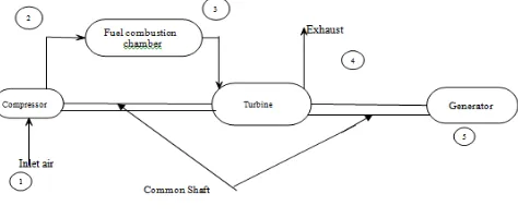
Each unit of

GTPPS consists of five main components, viz

turbine, compressor, combustion chamber,

Generator and electric system supporting the

whole unit. The various stages of operation are

shown in the Figure 1 as shown below.

Figure 1: Block Diagram of Single Shaft Gas Turbine Power Plant

The main components of the GTPPS plant is

described with following section.

(1) Compressor: The compressor in a GTPPS

power plant handle a large volume of air or

working media and delivering it at about 4 to

10 atmosphere pressure with highest possible

efficiencies The axial flow compressor is used

for this purpose. The kinetic energy is given to

the air as it passes through the rotor and part of

it is converted into pressure. The common types

of failures applicable in the compressor of

GTPPS system is as follows. (a) Exhaust

temperature high: (b) Air inlet differential

Trouble

(2) Combustion Chambers: The combustion

chamber perform the difficult task of burning

the large quantity of fuel, supplied through

the fuel burner with extensive volume of air

supplied by the compressor and releasing the

heat in such a manner that air is expanded and

accelerated to give a smooth stream of

uniformly heated gas at all conditions required

by the turbine. The common types of failures

applicable in the combustion chambers of

GTPPS system is as follows.(a) Loss of Flame.

(b) Servo Trouble:

(3) Gas Turbine: A gas turbine used in power

plant converts the heat and kinetic energy of the

gases into work The basic requirements of the

turbines are lightweight, high efficiency;

reliability in operation and long working life.

The common types of failures applicable in the

Gas Turbine component of GTPPS system is as

follows. (a) High Pressure (H.P) Turbine under

speed. (b) Low Pressure (L.P) Turbine Over

speed. (c) Wheel space differential temperature

high. (d) Mist eliminator Failure/Trouble. (e)

Turbine Lube Oil Header Temperature High. (f)

Low hydraulic pressure. (g) Bearing drain oil

temperature high:

(4)

International Journal of Emerging Technology and Advanced Engineering

558 (5) Electrical systems: The A.C. power circuit

ignition system receives an alternating current

that is passed through a transformer and

rectifier to charge a capacitor.

When the voltage in the capacitor is equal to

the breakdown value of a sealed discharge gap,

the capacitor discharges the energy across the

face of the ignition plug. Safety and discharge

resistors are fitted in the circuit. Except this

various circuit breakers, Relay system, Bus

Bars, control panels, transformers are used in

electrical systems. The main function is linking

the produced generation to hungry consumers‘.

The common types of failures found in the

Electrical systems of GTPPS system is as

follows

(a) De synchronization with Grid. The overall

Diagram of GTPPS Plant is described in

GTPPS operation diagram.

III.

A

RRANGEMENT

O

F

U

NITS

I

N

P

OWER

P

LANT

Before carrying out any research work understanding of the system is necessary. Block diagram of the system will help to understand the inner physics of any system. So a block diagram is necessary to understand the behavior of the system. Figure 2 represents the block diagram of Rukhia gas turbine Power plant. Proper planning is necessary to carry out any research work. For the repairable system analysis a flowchart of where to start, what are the things to do; a step by step working procedure is necessary. This Framework is presented in figure 3(Appendix B). In this framework a detailed working procedure and step by step model identification is presented.

(

Appendix A :

Figure 2 gives the GTPPS Operation Diagram of Rukhia Gas Turbine Power Plant.)

Methodology: In any Reliability analysis the identification of Proper model is necessary. As per the flow diagram the methodology for reliability modeling of Turbine, Compressor, Generator and Combustion Chamber and Electrical System consists of following steps

Step I: Identification of Relevant Parameters and Variables, and Collection of Relevant Data. Here all the failure data are collected as per the data

collection procedure. After that flow chart for reliability analysis is carried out. The different parameters and variables are identified and presented in the Parameters and variable sections. This detail descriptions is divided into three section

(a) Data collection

(b) Reliability Logic Diagram (c) Parameters and variables.

Data collection: The collection of Data is necessary to carry out the analysis. The data are collected from the maintenance logbook available in the plant and asking questions to the operators, supervisors and managers of the plant. Data are required to be collected over a period of time for providing satisfactory representation of the true failure characterization of the machine. Data used in recent studies have been collected for a period of 5 and half years. Approximately 956 failure data is collected for all the seven units over the stated Period. These Data are segregated according to component wise and unit wise. The failure time repair time and time of breakdowns reasons for failures are also collected.

(a) Reliability Logic Diagram:

Before carrying out any research work Understanding of the system is necessary. Block diagram of the system will help to understand the inner physics of any system. So a block diagram is necessary to understand the behavior of the system. Figure 3 represents the block diagram of Rukhia gas turbine Power plant. Proper planning is necessary to carry out any research work. For the repairable system analysis a flowchart of where to start, what are the things to do; a step by step working procedure is necessary. This Framework is presented in figure 3,and it is attached in Appendix A. In this framework a detailed working procedure and step by step model identification is presented. Parameters and variables.

Step-II: Component- and System-level Analysis

Decisions regarding relevance of component- or system-level analysis are to be taken on the basis of the following considerations. These considerations are taken under the heading of Component-level Analysis and System-level Analysis. The details of the analysis are described in the next section.

(5)

International Journal of Emerging Technology and Advanced Engineering

559

(normal or accelerated life tests) are to be conducted for such components for reliability analysis. Measurement and evaluation of reliability of such components would follow the analysis of test data.

(APPENDIX B : Figure 3 gives the Methodology for Reliability Analysis of turbine, compressor, combustion chamber and electrical system)

(c) Parameters and variables

The parameters of Turbine, Compressor, and Combustion chamber Generators are mentioned in Table 1 given in Appendix C.

IV. SYSTEM LEVEL ANALYSIS

For this kind of analysis, the configuration of the system as a whole is to be known. Both parametric as well as nonparametric approaches for reliability measurement and evaluation are a possibility. The conditions under which parametric or non-parametric approach is recommended are as follows:

Condition of Parametric approach: The number of data points related to a system is made available within the given time period and sufficient enough to verify the distributional assumption for the variables under consideration at an acceptable level of significance. A parametric approach may be applied in three situations: When the failure data follows a homogeneous Poisson process (HPP) (no trend and dependence in data), or (ii) nonhomogeneous Poisson process (NHPP) (trend in data), and (iii) Branching Poisson process (BPP) (no trend but dependence in data). The parameters of the three processes as mentioned may be estimated with a number of tools and techniques, such as ‗probability plot‘ and ‗maximum likelihood estimation‘

Conditions for Nonparametric Approach:

A nonparametric approach is recommended

when the following conditions are met. The

number of data points related to a system is

made available but insufficient enough to verify

the distributional assumptions for the variables

under consideration at an acceptable level of

significance. Special tools and techniques, such

as Kaplan-Meier estimator, simple and standard

actuarial methods, and regression analysis, are

used in this case.

The failure rate data of Turbine, Compressor, Combustion Chamber and Generator

may be analyzed with such techniques. In this case the trend test is done on the data and presented in the result section of trend test .

The electrical system follow the Renewal Process as dependency were not proved in the serial correlation tests. Hence Branching Poison Process is rejected.

Step III:

Development of Appropriate

Reliability Model. In this section the

appropriate reliability model is described

into following three sections.

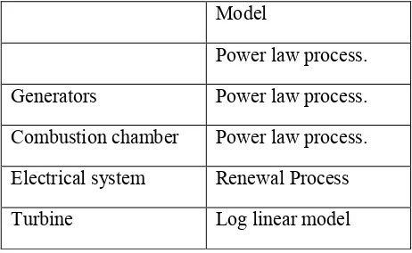
Statistical tests used: The statistical tests used here are trend test, serial correlation test, Laplace test and Military handbook tests. The procedure for carrying out all these tests are described in the Statistical tests and Reliability models section.

(a). Available reliability model: The different reliability models used here are Power law process and log linear process under the non homogenious poisson process and renewal process under the homogeneous poison process. The procedure for carrying out all these tests are described in the Statistical tests and Reliability models section. In addition the different reliability models and estimation of parameters and reliability estimation are described in the Statistical tests and Reliability models section. Selection of appropriate reliability model: The appropriate Reliability model is selected by different testing procedure as described in section (b), i.e. by Trend test , Serial correlation test, Military Handbook test and Laplace test, and renewal process. Based on the above test described in Result section the following conclusion is attained and described in table 2.

Model

Power law process.

Generators Power law process.

Combustion chamber Power law process.

Electrical system Renewal Process

[image:5.595.322.553.574.716.2]

Turbine Log linear model

(6)

International Journal of Emerging Technology and Advanced Engineering

560 Step IV: Verification and Validation of the

Proposed Approach.

The proposed models are to be tested for its

verification and validation in a number of

situations and conditions as discussed for the

testing Procedure. Modifications in the

proposed model are based on analysis of

difference between the actual and estimated

performance data over a period. The

methodology for reliability modeling of GTPPS

and its subsystems like turbine compressor,

combustion

chambers

and

Generators

considered to be a repairable system, is

explained in detail with the help of flow

diagram shown in Figure 3.This methodology is

applied for reliability analysis of GTPPS and its

subsystems

like

turbine

compressor,

combustion chambers and Generators and the

details of the application of methodology are

given below.

4. Statistical tests and Reliability models:

Various statistical tests are available for the

analysis of data. These are Trend tests, TTT

plot, Nelson Allen Plot, Serial correlation test,

Duane Growth model, Apart from for deciding

the appropriate reliability models the Military

handbook tests and Laplace stets are used. The

various Reliability models available are

homogeneous

poison

process,

non

homogenious poison process, branching

poisson process, renewal process and models

for non repairable items. The various statistical

tests and reliability models are described under

the following two sections described below (1)

statistical models (2) Reliability models

(1) Statistical Tests: The various Statistical

tests used in this paper are described below.

These are

Trend test- Cumulative failures verses

cumulative time between failures.

Serial Correlation test: to find whether Data is

independently and identically distributed.

Military Handbook test: To find the data pattern

follow Power law process

Laplace test: To find out the data pattern follow

Log linear process .All these aforesaid tests are

stated below.

Trend Test:-

The graphical trend test and

serial correlation test of TBF data of Turbine ,

compressor, Generator, combustion chamber

and electrical components and their subsystems

are necessary for validity of assumption that

failure data are independently distributed (iid)

in an analysis of failure distribution model. The

trend test is done by plotting the cumulative

time

between

failure

(CTBF)

against

cumulative frequency of occurrence. Serial

correlation test is done by means of plotting ith

TBF against (i-1) th TBF. Trend plot of

Turbine, compressor, Generator, combustion

chamber and electrical components and their

subsystems will be five curves presented in

figure.. In the test, weak or absolute trends were

found for Turbine, compressor, Generator,

combustion chamber and no trend in electrical

components and exhibited concave upward and

concave downward respectively in trend

test..The trend test were further elaborated by

Trend test 1 and Trend test 2 in Reliability

modeling to determine Homogeneous poison

process or Non Homogeneous poison process in

trend test 1 and Renewal process or Non

Renewal Process in Trend test 2 Finally the

Reliability of each system are calculated by

selecting the Proper model in analysis and the

models are followed in the manner as described

below.

Serial Correlation test:

Serial correlation test

is done by means of plotting ith TBF against

(i-1) th TBF. The condition is = Points are not

randomly scattered and in straight line . *Data

are dependent and Branching Poison Process

can be applied . Points are randomly scattered

and not in straight line ≠ Data have no

correlation and dependence = Data are

independent and identically Distributed.

(7)

International Journal of Emerging Technology and Advanced Engineering

561 serial correlation test, the points are randomly

scattered not in a straight line. For example,

serial correlation test of Turbine, compressor,

Generator, combustion chamber and electrical

components are presented in different figures.

So the above failure data can be assumed to be

independently and identically distributed (iid)

Military Hand book test:

The Military Handbook test is a test for the

null hypothesis

H₀ :HPP

versus alternative

hypothesis

H

₁

:

NHPP

with increasing power

law process. The test statistic of this test for

more than one process is given by

ˆ

1 1

2 i ln( )

n m

i i

C

i j ij i

b a

M

t a

 

 





---

(22)

And it is chi-square distributed with 2q degrees

of freedom,

Where





 m

i i

n q

1

ˆ

under the null hypothesis of

HPP [Kvaloy and Lindquist, 1998]. The Mc

value is calculated corresponding to failure

parameters of component and compared with

chi square value of 2N degree of freedom and

if chi square value is > than Mc value than

Null hypothesis is rejected otherwise Null

hypothesis is accepted. thus deciding Log linear

model or Power law process. In case the null

hypothesis is not accepted for both the tests,

then the conflict regarding NHPP with

log-linear model or power law process is resolved

by calculating the so-called probability or

P-values of the tests as mentioned. The P-value

for a normal distribution is defined to be the

probability value corresponding to the z-value

against Laplace‘s test statistic. For Military

Handbook test, P-value corresponds to the χ

2

-value with one degree of freedom. A smaller

P-value is indicative a stronger evidences a null

hypothesis [Rigdon and Basu, 2000][32].

Laplace test:- Laplace‘s test is conducted for

the null hypothesis,

H₀ :HPP

versus the

alternative hypothesis,

H

₁

:

NHPP

with

log-linear model. The generalization of the

Laplace‘s test statistic for more than one

process may be given by

ˆ

1 1 1

2

1 1

ˆ ( )

2 1

ˆ ( )

12

i

n

m m

ij i i i

i j i

C _m

i i i

i

t n b a

L

n b a

  



 





 



---

(23)

Where

n

ˆ = n or (n-1) if the process is time

_i

truncated or failure truncated, respectively

[Kvaloy and Lindquist, 1998].[33] This test

statistic is asymptotically standard normally

distributed under the null hypothesis. The

Laplace

statistics

value

is

calculated

corresponding to failure parameters of

component and compared with chi square

value of N degree of freedom and if chi square

value is < than the Laplace value than Null

hypothesis

is

rejected

otherwise

Null

hypothesis is accepted. thus deciding Log linear

model or Power law process. (2) Reliability

models: The various Reliability models used in

this paper are described below. These are

Homogeneous

Poisson

Process,

Non

homogeneous Poisson Process,

and Branching Poison Process,

Renewal Process and Non repairable

items

Homogeneous Poisson Process

The homogeneous Poisson process is a Poisson

process with constant intensity function

[Rigdon and Basu, 2000][11]. Since the

systems are identical, the failure process of

each system is an HPP with intensity



1

, and



is same for all systems. A counting process is a

homogenous Poisson process with parameter λ

>0 if :

N

(0)=0. The process has independent

increments

The number of failures in any interval of length

(8)

International Journal of Emerging Technology and Advanced Engineering

562 F(t) = 1- e

-λt

= The cumulative density

function of the waiting time to the next failure

(or interarrival time between failures)

N(T) = the cumulative number of failures from

time 0 to time T. P{N(t)=k} = (λT)

k

e

-λt

/ k│

M (T) =λt = the expected number of failures by

time T, λ = the rate of occurrence of failure

ROCOF, 1/λ = The Mean time between

failures (MTBF). So the reliability R(t) in the

case of Homogeneous Process =- e

-λt

---(1)

Branching Poison Process:

Figure: 4 Example of Branching Process, Ref [12]

The Branching Poison Process: In some cases

failures tend to be bunched together . This may

indicate that the system is not correctly repaired

causing a number of subsequent failures. A

model that can account the phenomenon is the

branching Poisson Process (BPP). The BPP was

originally proposed by Bartlett (1963)[13] as a

model for Traffic flow., where a slow moving

vehicle may be followed immediately by a

number of other vehicles. This is analogous to

to a single failure causing a number of

subsequent failures. Lewis (1965)[14] applied

the BPP to failure times of computers. To be

more precise suppose the primary failures are

generated according to poison process with rate

λ . After each failure there is probability 1-r that

the repair will be done correctly; In this case

the next failure will occur when the next

primary failures occurs. With probability r, the

repair is not done correctly; In this case the

primary failure will spawn a finite renewal

process of subsidiary failures.

The number of of subsidiary failures that follow

from a primary failure is a discrete random

variable. Lewis (1964) and cox and Lewis

(1966)[15,16] describe the cases where the

random variable has a geometric, negative

binomial and poison distribution. It is assumed

that both kind of failures (primary and

secondary) are indistinguishable. Define G to

be the number of subsidiary failures

corresponding to a single primary failure

conditioned on there being at least one such

subsidiary failures and let S be the

(unconditional) number of subsidiary failures.

Note that S=0 when the repair is done correctly.

Let Z1, Z2 ---- denote the times between the

primary failures and let Y

i (1),

Y

i

(2),---Y

i(s),

times between the subsidiary failures

that are triggered by ith primary failures.

Finally let T

1

< T

2

< T

3

denotes the failure time

regardless of the type. In practice we observe

only the Ti‘s and not the type of failure. The

ROOCOF function for the BPP can be obtained

as follows. Let H(t) denote the expected

number of subsidiary failure from a single

primary failure to an interval interval of length

t and let F

k

(t) and f

k

(t) denote the cdf and pdf

respectively of the random variable Z

1

+ Z

2

+---+ Z

k

(i.e. the time of the k th primary

failure) Given that Z

1

=z the expected events in

the interval[0,t] from the first subsidiary

process, the first subsidiary process, then E[N

(1)

_{(t) the number of failures in (0,t) due to first}

subsidiary process then

E[[N

(1)

(t)]=

E{

N

(1)

(t)│Z

1

]}

=

∫

(t)ІZ

2

=z] f

1

(z) dz

=

∫

(z)dz

A similar analysis could be applied to the time

of the k th failure. The expected no of failure N

(1)

_{(t) in (0,t) due to the kith subsidiary process is}

(9)

International Journal of Emerging Technology and Advanced Engineering

563 The expected number of failure of any type in

[0,t] is thus Λ(t) =E[N,(t)]=E( Number of

Primary

failure

in

[0,t])

+

∑

from

k th primary failure)

= Λz(t) +

∑

∫

= Λz (t) +

∫ ∑

(z)]dz

= Λz (t) +

_∫

(z) dz----[3}

The ROCOF for the branching process is

therefore

=Λ(t). =Λ

z

(t) + d/dt

∫

zdz. .If no subsidiary failure is there the

ROCOF

=λ--- (2)

The Reliability function is = e

-λt

Renewal Process: RP is defined as a process in which the different times to failure of a component or system, Xi, are considered independently and identically distributed random variables. This is consistent with the primary underlying notion of this process that assumes that the system is restored to its original (like new) condition following a relatively instant repair action. Because it represents an ideal situation, this model has very limited applications in the analysis of repairable systems, unless the system consists of primarily non-repairable (replaceable) components in sockets. That is, when a part of the system fails, it will be taken out and replaced by a new one [17] . The expected number of failures in a time interval [0, t] is given by: Λ (t) = F(t) +∫

---(3)

Where F (t) is the cumulative distribution function (cdf) of the time between successive repairs or replacements of the system. By taking the derivative of both sides of Eq. (1) with respect to t:

λ(t) = f(t) + ∫

---(4) Where f(t ) is the probability density function (pdf) of the time between successive failures. In case of the two parameter Weibull distribution, representing the random variable t, the cdf and the pdf are of the form:

F (t) = 1- --- (5)

F (t) =

--- (6)

Where a and b are the scale and shape parameters, respectively. The ML estimators for parameters a and b are [18,19]:

=

[

∑

_]

---

(7)

∑

[

]

∑

--

^

=

∑

--- (8)

Where ti is the observed time between successive failures and n is the total number of failures observed. A close form solution to estimate the expected number of failures in the case of Weibull distribution has not been developed yet. Instead, a group of numerical solutions can be obtained. Smith and Lead [20] better have proposed an iterative solution to the renewal equation for cases where the failure interarrival times follow a Weibull distribution.

The maximum likelihood estimation is done by and β¯ and Reliability is estimated by the formula

= --- (9)

Non repairable item

For this model illustrated in figure 3. there is neither preventive maintenance nor corrective nor preventive maintenance, and the failure intensity equals 0 after failure has occurred. The component history (step 2) is recorded by X(t), where

X(i) =1, if i<X, and 0 otherwise--- (10) The variable Keeps track of whether the failure has occurred or not, which is the only event relevant to IC(t)The intensity process IC(t) (step 3) is

(10)

International Journal of Emerging Technology and Advanced Engineering

564

Thus the intensity process is the hazard rate of the inherent TTF, truncated at time of failure and I(t) –E[ IC(t) –E[λ(t),X(t)]= λ(t).E[X(t)]= λ(t).R(t) =f(t)

–---(12)

This is a special case of eqn(12) and again gives the result that the mean intensity, I(t), for a nonreplicable items equals the pdf, f(t). The interpretation is that at time [t,t+dt) equals f(t). dt

Nonhomogenious Poison Process:

Nonhomogeneous Poisson processes are also useful for modeling repairable system reliability [Bertkeats and Chambal, 2002; Ryan, 2003].[21,22] The failure process between two successive overhaul actions is described by a nonhomogeneous process [Ascher and Feingold, 1984; Engelhard and Bain, 1986][23,24]. The NHPP model also assumes ‗minimal repair‘, which means that after each failure and following repair, the system is in the same state as it was just prior to that failure [Heggland and Lindqvist, 2007][25]. Moreover, it is also assumed that the failed part is small one of the system. During and after repair or replacement of this part the other parts will not be affected. The assumption for modeling of more than one system is that all systems are identical with respect to their technology and mean time between failures. Also, all systems are time-truncated with same starting and finishing points. Among the NHPP‘s, large attention has been devoted to the power law process [Walls and Bendell, 1986; Pulcini, 2001] [26,27] and log-linear processes [Cox and Lewis, 1966; Baker, 2001].[28,29] In this context, it is mentioned that if the failure data of a system rejects the null hypothesis of Laplace‘s Test, the data is considered to follow the log-linear model. On the other hand, if the failure data of a system rejects the null hypothesis of Military Handbook test, the data follows the power law model. The following sections describe the procedures for estimation of parameters for the two models (Power Law and Log-linear Processes), as mentioned.

Power Law Process

The intensity function of power law process is

given as follows [Crow, 1990]:[30].

 

_t

 1



_



 _{, λ where,}__,__{, t > 0, and t is the}

age of the system. Hence, the power law mean value function is given by,

( ( )) , t 0

E N t 



t  ---(13)

The probability that a particular system will experience n failures over its age (0, T) is given by the Poisson expression [Rigdon and Basu, 1989][31],

(

)

( ( )

)

, n 0, 1, 2,...

!

n T

T

e

P N t

n



 







----14)

And the reliability may be given by, R(t) = exp{intensity function -λt}. Maximum likelihood estimation of the parameters may be described as follows: Let, tij denotes the jth failure of ith system.

Suppose, ni failures are observed for system i.

Applying the joint pdf theorem, the MLE of parameters of power law process is given by and estimated as stated. Hence, the intensity function of power law process for GTPPS -unit is given .With the help of this intensity function the reliability of the GTPPS -unit may be calculated

1

ˆ

k i i k

in i

n

t 

 



 



--- (15)

and 1

1 1 1

ˆ

ˆ _{log( )} i _{log( )}

k i i

n

k k

in in ij

i i j

n

t  t t

 



  

 







--(16)

If the systems are time-truncated and tin=T for all

systems, the above-mentioned estimates may be written as

1

ˆ

k i i

n

kT

_



 _{--- (17)}

and

1

1 1

ˆ

log( )

i

k

i i n k

i j ij

n

T t

 

 

 





---(18) (18)

Reliability R(t) = e –intensity function Log Linear Model

(11)

International Journal of Emerging Technology and Advanced Engineering

565 ( )

t

e

 t



_

 _{--- (19)}

Where , , t>0, and t is the age of the system. Similar to power law process the maximum likelihood estimates of parameters of log-linear process for more than one system is calculated as follows

ˆ 1

ˆ

(

1)

k

i i

T

n

e

k e















---(20) (20)

and

ˆ

1 1

ˆ 1 1

0 ˆ

₍

₁₎

i

k k T i i n

k

i i ij _T i j

n

Te

n

t

e



 















-

(21)

Reliability R(t) = e –intensity function

V. RESULTS

Data used in recent studies have been

collected for a period of 5 and half years.

Approximately 956 failure data is collected for

all the seven units over the stated Period. These

Data are segregated according to component

wise and unitwise.The failure time repair time

and time of breakdowns reasons for failures are

also collected. These failure data of different

units were collected from the maintenance log

book. Failure behavior of these machines has an

influence on availability or failure pattern of the

machine as a whole. The basic methodology for

reliability modeling is presented in figure 3. It

shows a detailed flow chart for model

identification and is used here as a basis for the

analysis of failure Data So TBF are arranged in

a chronological order for using statistical

analysis to determine the trend in failure and

other aspects of Reliability. In this section the

detail analysis of the test carried out on

different components are discussed.

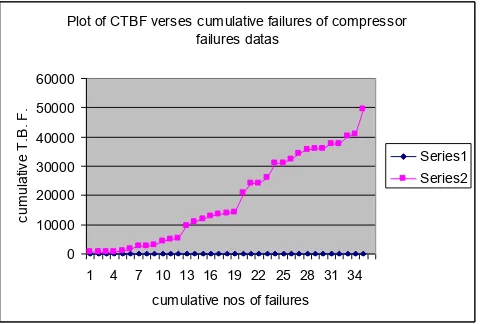
Compressor: The Cumulative TBF verses

cumulative failures datas are drawn in a plot

and the plot is shown below in figure 5.

Similarly the failure Data of ith failure verses

(i-1) th failure data are plotted in figure 6.

The result shows that Failure data line has

slight deviation from straight line. and

the points

[image:11.595.318.558.167.329.2]

are randomly scattered and not in straight line in the serial correlation test.

[image:11.595.316.557.362.520.2]

Figure :-5 Cumulative Failure nos verses cumulative time between failure Data of compressor system

Figure: 6 Serial correlation test of Compressor units of GTPPS.

Conclusion: Data is modeled by NHPP.and data are independently and identically distributed. Now to select the model for Log linear or Power law process the data are further processed by carrying out military Handbook Test. The result of Military Handbook Test is described in table 2.

It is mentioned that if the failure data of a system rejects the null hypothesis of Laplace‘s Test, the data is considered to follow the log-linear model. On the other hand, if the failure data of a system rejects the null hypothesis of Military Handbook test, the data follows the power law model. Data Pattern follow the Power Law Process. By applying the Formula of intensity function and appropriate formula of Reliability the Reliability at different time intervals are calculated and it is shown graphically in the figure 7 mentioned below.

Plot of CTBF verses cumulative failures of compressor failures datas

0 10000 20000 30000 40000 50000 60000

1 4 7 10 13 16 19 22 25 28 31 34 cumulative nos of failures

cu

m

ul

at

iv

e

T

.B.

F

.

Series1 Series2

Serial Corelation test of compressor failure Datas

0 5000 10000

0 5000 10000 ( i -1)th T.B.F

I t

h

T

.B.

F

.

(12)

International Journal of Emerging Technology and Advanced Engineering

[image:12.595.316.562.114.470.2]

566

Table: 2 Result of Military Handbook test of Compressor

[image:12.595.315.564.128.278.2]

Figure 7 Reliability at different intervals of compressor units.

Table: 3 Result of Military Handbook test of Combustion Chamber

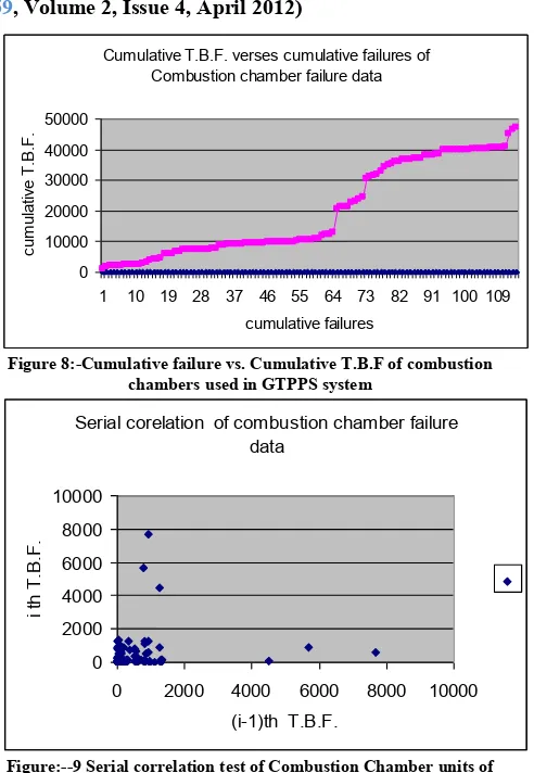
Combustion Chamber: The Cumulative TBF verses cumulative failures datas are drawn in a plot and the plot is shown below in figure 8. Similarly the failure Data of ith failure verses (i-1) th failure data are plotted in figure 9. The result shows that Failure data line have slight deviation from straight line. and the points are randomly scattered and not in straight line in the serial correlation test.

Figure 8:-Cumulative failure vs. Cumulative T.B.F of combustion chambers used in GTPPS system

Figure:--9 Serial correlation test of Combustion Chamber units of GTPPS.

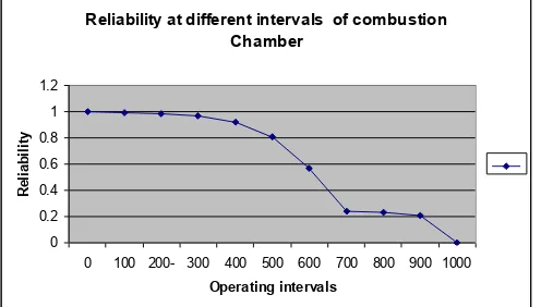
Conclusion: Data is modeled by NHPP.and data are independently and identically distributed. Now to select the model for Log linear or Power law process the data are further processed by carrying out military Handbook Test. The result of Military Handbook Test is as follows. It is mentioned that if the failure data of a system rejects the null hypothesis of Laplace‘s Test, the data is considered to follow the log-linear model. On the other hand, if the failure data of a system rejects the null hypothesis of Military Handbook test, the data follows the power law model. Data Pattern follow the Power Law Process. By applying the Formula of intensity function and appropriate formula of Reliability the Reliability at different time intervals are calculated. and it is shown graphically in the figure 10 mentioned below.

Reliability at different intervals of Compressor

0 0.1 0.2 0.3 0.4 0.5 0.6 0.7 0.8 0.9 1

0 100 200- 300 400 500 600 700 800 900 1000

operating Time

R

el

ia

bi

li

ty

Cumulative T.B.F. verses cumulative failures of Combustion chamber failure data

0 10000 20000 30000 40000 50000

1 10 19 28 37 46 55 64 73 82 91 100 109

cumulative failures

cu

m

ul

at

iv

e

T

.B.

F

.

Serial corelation of combustion chamber failure data

0 2000 4000 6000 8000 10000

0 2000 4000 6000 8000 10000 (i-1)th T.B.F.

i t

h

T

.B.

F

.

Compon ent

MC

value

Sam ple size

Χ2 N,,0.5val

ue

Result

Compre ssor

-30.354

35 Χ2

35,,0.5=4

5.5

Null hypothesis rejected

Compon ent

MC

valu e

Samp le size

Χ2

N,,0.5valu

e

Result

Combust ion Chamber

-104. 3

60 <Χ2 60,,0.5=

88.38

[image:12.595.49.292.134.378.2] [image:12.595.40.296.422.508.2]

(13)

International Journal of Emerging Technology and Advanced Engineering

[image:13.595.321.561.128.284.2]

567

Figure 10: Reliability at different intervals of combustion chamber system.

Generator:

The Cumulative TBF verses

cumulative failures data are drawn in a plot and

the plot is shown below in figure 11. Similarly

the failure Data of I th failure verses (i-1) th

failure data are plotted in figure 12. The result

shows that Failure data line has slight deviation

from straight line. and the points are randomly

scattered and not in straight line in the serial

correlation test.

[image:13.595.50.298.131.272.2]

Figure 11:-Cumulative failure vs. Cumulative T.B.F of Generators used in GTPPS system

Figure 12: Serial correlation tests of Generator units of GTPPS.

[image:13.595.302.555.405.471.2]

Conclusion: data is modeled by NHPP.and data are independently and identically distributed. Now to select the model for Log linear or Power law process the data are further processed by carrying out military Handbook Test. The result of Military Handbook Test is as follows

Table 4: Result of Military Handbook test of Generator

Conclusion: Data Pattern follow the Power Law Process. By applying the Formula of intensity function and appropriate formula of Reliability the Reliability at different time intervals are calculated. and it is shown graphically in the figure 13 mentioned below

Figure: 13 Reliability at different intervals of Generator system

Reliability at different intervals of combustion Chamber

0 0.2 0.4 0.6 0.8 1 1.2

0 100 200- 300 400 500 600 700 800 900 1000

Operating intervals

R

el

ia

bi

li

ty

Plot of cumulative T.B.F. verses cumulative failures of Generator failure data

0 10000 20000 30000 40000 50000 60000

1 6 11 16 21 26 31 36 41 46 51 56 61 66 71 76 81 cumulative failures

cu

m

ul

at

iv

e

T

.B

.F

.

Serial corelation test of Generator system failure data

0 1000 2000 3000 4000 5000 6000 7000

0 2000 4000 6000 8000

(i-1)th T.B.F.

I

th

T

.B

.F

.

Series1

Reliability at different operating intervals of Generator

0 0.2 0.4 0.6 0.8 1

100 200- 300 400 500 600 700 800 900 1000

Operating time

R

el

ia

bi

li

ty

Compon ent

MC

value Sam ple size

Χ2 N,,0.5val

ue

Result

Generat or

-46.85 60 Χ2 60,,0.5=8

8.38

Null hypothesis rejected

Compone nt

MC

value

Sampl e size

Χ2

N,,0.5valu

e

Result

Generator -46.85 60 Χ2

60,,0.5=88.

38

[image:13.595.46.290.437.672.2] [image:13.595.318.563.585.725.2]

(14)

International Journal of Emerging Technology and Advanced Engineering

568

Turbine: The Cumulative TBF verses cumulative failures data are drawn in a plot and the plot is shown below in figure 14. Similarly the failure Data of ith failure verses (i-1) th failure data are plotted in figure 15. The result shows that Failure data line has slight deviation from straight line. and the points are randomly scattered and not in straight line in the serial correlation test.

[image:14.595.310.558.214.333.2]

Figure 14:-Cumulative failure vs. Cumulative T.B.F of Turbines used in GTPPS system

Figure: 15 Serial correlation test of Turbine units of GTPPS.

Conclusion: data is modeled by NHPP.and data are independently and identically distributed. Now to select the model for Log linear or Power law process the data are further processed by carrying out military Handbook Test and Laplace test.. The result of Military Handbook Test is Null hypothesis is accepted It is mentioned that if the failure data of a system rejects the null hypothesis of Laplace‘s Test, the data is considered to follow the log-linear model.

On the other hand, if the failure data of a system rejects the null hypothesis of Military Handbook test, the data follows the power law model. Since Turbine failure Data rejects the Null hypothesis in Laplace test the failure Data follows Log Lineaer model. The result of Laplace Test is as follows

Com pone nt

Laplu s Statist ics

LC>0 or LC< 0

Laplace Statistics> <chi square statistics Χ2N,,0.5

Null Hypot hesis

Turb ine

-111.9 3

LC<0,

decreasing trend

> Χ2

N,,0.5 Reject

[image:14.595.319.573.450.598.2]

ed

Table: 5 Result of Laplace test of Turbine unit system.

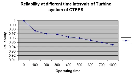
Conclusion: Data Pattern follow the Log linear model.By applying the Formula of intensity function and appropriate formula of Reliability the Reliability at different time intervals are calculated. and it is shown graphically shown in the figure 16 as mentioned below

Figure16: Reliability at different intervals of Turbine system

Electrical System: The Cumulative TBF verses cumulative failures datas are drawn in a plot and the plot is shown below in figure 17. Similarly the failure Data of ith failure verses (i-1) th failure data are plotted in figure 18. The condition is Deviations from straight line: trend is absent No deviations – trend present, Points are randomly scattered and not in straight line .

Data are independent and identically distributed. In straight line = Data have correlation and dependence.

Plot of cumulative failures verses cumulative T.B.F. of Turbine system failure

0 10000 20000 30000 40000 50000 60000 70000 80000

1 26 51 76 101 126 151 176 201 226 cumulative failures

C

um

ul

at

iv

e

T.

B

.F

.

Series1 Series2

Serial corelation test of Turbine system failure data

0 500 1000 1500 2000 2500 3000 3500

0 1000 2000 3000 4000 (i-1)th TBF

It

h

T

B

F

Series1

Reliability at different time intervals of Turbine system of GTPPS

0.91 0.92 0.93 0.94 0.95 0.96 0.97 0.98 0.99 1

0 100 200 300 400 500 600 700 1000

Operating time

R

el

ia

bi

li

[image:14.595.52.294.450.607.2]

(15)

International Journal of Emerging Technology and Advanced Engineering

[image:15.595.49.299.123.429.2]

569

Figure 17: Cumulative failure vs. Cumulative T.B.F of electrical system used in GTPPS system

Figure18: Serial correlation tests of Electricals system units of GTPPS.

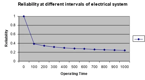
Conclusion: Trend is absent Hence it is Homogeneous Process Since correlation and dependence is absent Datas are independently and identically distributed. So next condition is after repair it is as good as new. Yes it is as good as new so this is a case of Renewal Process .By applying the Formula of intensity function and appropriate formula of Reliability the Reliability at different time intervals are calculated and it is shown graphically shown in the figure 19 as mentioned below

Figure19: Reliability at different intervals of Electrical system

Reliability analysis in system level:-

Estimation of Reliability of systems by using the Reliability of components.

Unit Level Reliability: Assuming the total System has identical units and all the 5 units are parallally connected keeping two standby units as shown in the operational Diagram of GTPPS. The unit and System level Reliability is calculated. Unit level Reliability: Since all the components are in series the series system reliability is Rs= R1x R2x R3x R4x

R5 [34] the system level reliability is calculated by

[image:15.595.49.301.132.253.2]

applying the series level formula. The Calculated Reliability is shown in the Graph of figure 20.

Figure 20: Reliability at different intervals of identical units in series system.

Determination of Parallel system Reliability: Parallel Using the Formula Rp=1-Qp 1-[1-e(-λt))]n

[36]of Parallel system Reliability we get the Reliability of Parallel system at different time intervals. The Reliability at different time intervals and is shown in Figure 21.

Figure 21: Reliability Pattern of Parallel system unit failure Dataˆˇ Cumulative T.B.F. verses cumulative failure data of electrical

system failures

0 100000 200000 300000 400000 500000 600000

1 14 27 40 53 66 79 92 105 118 131 144 157 170

cumulative failures

cu

m

ula

tiv

e

T.

B.

F.

Serial corelation test of electrical system failure data

0 1000 2000 3000 4000 5000 6000

(i-1) th T.B.F.

ith

T

.B

.F

.

Reliability of Parallel unit from unit 1,4,5,6,8 units in GTPPS

0 0.2 0.4 0.6 0.8 1

0 100 200- 300 400 500 600 700 800 900 1000 Operating Time

R

el

ia

bi

li

ty

Reliability Pattern of the GTPP system having all units in parallel

0 0.1 0.2 0.3 0.4 0.5 0.6 0.7 0.8 0.9 1

0

100 _200- 300 400 500 600 700 800 900 ₁₀₀₀ Operating Time

R

el

ia

bi

lit

y

Reliability at different intervals of electrical system

0 0.2 0.4 0.6 0.8 1

0 100 200 300 400 500 600 700 800 900 1000

Operating Time

R

e

lia

b

ili

[image:15.595.50.293.613.747.2]

(16)

International Journal of Emerging Technology and Advanced Engineering

570 Determination of standby system Reliability

The formula used here is

,Rs(t) = λ1t +

λ1t_- λ2t_{)+ λ} 1 λ2

X[

+

]

[35]---[27] Where

λ1 = Failure rate of the Parallel units

λ2 = Failure rate of the standby unit

λ3 = Failure rate of the second standby unit

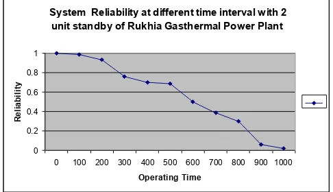
[image:16.595.47.286.132.322.2]

Using the appropriate formula we got the Parallel system reliability with two unit standby. The Reliability at different time interval is shown in figure 22

Figure 22: Reliability Pattern of whole plant unit if two stand by unit is kept

6.0 Discussion:-The selection of model for calculation of Reliability shows that the turbine unit follows Log Linear model and compressor unit, Generator and combustion chamber units follows Power law model and electrical system follow Renewal Process. The Reliability of different components of Rukhia Gas Power Plant is analyzed by taking the failure data of different operating units and consultation with Plant operating Personnel and management People about the arrangement of units in winter and summer season, It is known that in winter less Power is supplied to Grid and two units are kept as standby system. In Summer the demand is more and only one unit is kept as standby system. In both cases Reliability is determined by taking one and two units as stand by. Initially the component level Reliability is discussed one by one.

Compressor: The trend test shows that there is little deviations from straight line. So it can be concluded that Data Pattern of TBF data have trend.

In serial correlation test it is proved that Data pattern are independently and identically distributed. So Data are modeled by Non Homogeneous Poison Process Now for deciding whether Data Pattern follow the Power l;aw process or Log Linear model Data are again tested by Military Handbook test. It is Proved that the Data Pattern follow the Power law Process as Null hypothesis is rejected in Military Handbook test. By setting the Parameters of Power law Process the Reliability at different time interval are shown in figure 7. The Reliability from 0th hour to 100 th hour is drastically changing in the Diagram.

Combustion Chamber: The trend test shows that there is little deviations from straight line. So it can be concluded that Data Pattern of TBF data have trend. In serial correlation test it is proved that Data pattern are independently and identically distributed. So Data are modeled by Non Homogeneous Poison Process Now for deciding whether Data Pattern follow the Power l;aw process or Log Linear model Data are again tested by Military Handbook test. It is Proved that the Data Pattern follow the Power law Process as Null hypothesis is rejected in Military Handbook test. By setting the Parameters of Power law Process the Reliability at different time interval are shown in figure 10. Here the Reliability is almost constant fro 0 th hour to 200 hour and from 700 hour to 900 hour which requires further investigation as Reliability pattern does not show a constant Path.

Generator: The trend test shows that there is little deviations from straight line. So it can be concluded that Data Pattern of TBF data have trend. In serial correlation test it is proved that Data pattern are independently and identically distributed. So Data are modeled by Non Homogeneous Poison Process Now for deciding whether Data Pattern follow the Power l;aw process or Log Linear model Data are again tested by Military Handbook test. It is Proved that the Data Pattern follow the Power law Process as Null hypothesis is rejected in Military Handbook test. By setting the Parameters of Power law Process the Reliability at different time interval are shown in figure 13. Here the Reliability Pattern shows a decreasing trend with constant rate. It is almost acceptable..

Turbine: The trend test shows that there is little deviations from straight line. So it can be concluded that Data Pattern of TBF data have trend.

System Reliability at different time interval with 2 unit standby of Rukhia Gasthermal Power Plant

0 0.2 0.4 0.6 0.8 1

0 100 200 300 400 500 600 700 800 900 1000

Operating Time

R

el

ia

bi

li

[image:16.595.48.291.351.491.2]