Bunce, E.J. and Grodent, D.C. and Jinks, S.L. and Andrews, D.J. and
Badman, S.V. and Coates, Andrew J. and Cowley, S.W.H. and Dougherty,
M.K. and Kurth, W.S. and Mitchell, D.G. and Provan, G. (2014) Cassini
nightside observations of the oscillatory motion of Saturn’s northern auroral
oval. Journal of Geophysical Research: Space Physics 119 (5), pp.
3528-3543. ISSN 2169-9380.
Downloaded from:
Usage Guidelines:
Please refer to usage guidelines at
or alternatively
Cassini nightside observations of the oscillatory
motion of Saturn
’
s northern auroral oval
E. J. Bunce1, D. C. Grodent2, S. L. Jinks1, D. J. Andrews3, S. V. Badman4, A. J. Coates5,6, S. W. H. Cowley1, M. K. Dougherty7, W. S. Kurth8, D. G. Mitchell9, and G. Provan1
1
Department of Physics and Astronomy, University of Leicester, Leicester, UK,2Laboratory for Planetary and Atmospheric Physics, University of Liège, Liège, Belgium,3Swedish Institute of Space Physics-Uppsala, Uppsala, Sweden,4Department of Physics, Lancaster University, Lancaster, UK,5Mullard Space Science Laboratory, University College London, Dorking, UK, 6Centre for Planetary Sciences at UCL/Birkbeck, London, UK,7Blackett Laboratory, Imperial College, London, UK, 8
Department of Physics and Astronomy, University of Iowa, Iowa City, Iowa, USA,9Applied Physics Laboratory, Johns Hopkins University, Laurel, Maryland, USA
Abstract
In recent years we have benefitted greatly from thefirst in-orbit multi-wavelength images of Saturn’s polar atmosphere from the Cassini spacecraft. Specifically, images obtained from the Cassini UltraViolet Imaging Spectrograph (UVIS) provide an excellent view of the planet’s auroral emissions, which in turn give an account of the large-scale magnetosphere-ionosphere coupling and dynamics within the system. However, obtaining near-simultaneous views of the auroral regions with in situ measurements of magneticfield and plasma populations at high latitudes is more difficult to routinely achieve. Here we present an unusual case, during Revolution 99 in January 2009, where UVIS observes the entire northern UV auroral oval during a 2 h interval while Cassini traverses the magneticflux tubes connecting to the auroral regions near 21 LT, sampling the related magneticfield, particle, and radio and plasma wave signatures. The motion of the auroral oval evident from the UVIS images requires a careful interpretation of the associated latitudinally“oscillating”magneticfield and auroralfield-aligned current signatures, whereas previous interpretations have assumed a static current system. Concurrent observations of the auroral hiss (typically generated in regions of downward directedfield-aligned current) support this revised interpretation of an oscillating current system. The nature of the motion of the auroral oval evident in the UVIS image sequence, and the simultaneous measured motion of thefield-aligned currents (and related plasma boundary) in this interval, is shown to be related to the northern hemisphere magnetosphere oscillation phase. This is in agreement with previous observations of the auroral oval oscillatory motion.1. Introduction
The highly inclined orbits of the Cassini spacecraft at Saturn have provided thefirst opportunity to sample the coupled solar wind-magnetosphere-ionosphere system through the direct measurement of the associated high-latitudefield-aligned current systems. Where these high-latitudefield-aligned currents are directed upward away from the planet along magneticfield lines toward the magnetosphere, electrons are accelerated downward toward the ionosphere and are ultimately responsible for the production of the main auroral emissions at Saturn [Bunce et al., 2008;Talboys et al., 2009a, 2009b, 2011]. While the details of the driving physical mechanism and modulation of Saturn’s high-latitudefield-aligned current systems and thus main auroral emission are still under investigation, it has been shown that the upwardfield-aligned currents map to the outer magnetosphere, and are therefore likely to be associated with theflow shear between open (or at least very long, closed tailfield lines—see discussion in section 2) and closed outer magnetosphere magneticfield lines rather than being directly due to the breakdown of plasma corotation due to mass loading [Bunce et al., 2008;Talboys et al., 2011]. This is in broad agreement with the modeling work proposed byCowley et al.[2004a, 2004b, 2008], where the solar-wind interaction was suggested to be the driving mechanism producing the main auroral emissions at Saturn. However, in order to fully understand the details of the dominant mechanism, in situ observations of thefield-aligned current systems are ideally studied with contemporaneous imaging of the auroral emissions themselves. In order to obtain a“global”view of the high-latitude regions, the Cassini remote sensing instruments typically observe from, or close to, apoapsis (i.e., ~25–30 Rsfrom the planet during the 2008/9 orbits). Conversely, the associatedfield-aligned current
Journal of Geophysical Research: Space Physics
RESEARCH ARTICLE
10.1002/2013JA019527Key Points:
•First joint UV and in situ measurements of Saturn’s nightside northern aurora
•Motion of auroral oval allows detailed analysis of thefield-aligned currents
•Motion is due to the NH magneto-sphere oscillation phase
Correspondence to:
E. J. Bunce,
emma.bunce@ion.le.ac.uk
Citation:
Bunce, E. J., et al. (2014), Cassini night-side observations of the oscillatory motion of Saturn’s northern auroral oval,J. Geophys. Res. Space Physics,119, 3528–3543, doi:10.1002/2013JA019527. Received 22 OCT 2013
Accepted 20 APR 2014
Accepted article online 28 APR 2014 Published online 16 MAY 2014
signatures are most clearly observed when the spacecraft is much closer to the planet at periapsis (i.e., ~3–8 Rs from the planet). Thus, during the inclined orbit phase of 2008/9, there have been relatively few opportunities to combine near-simultaneous auroral imaging from the Cassini remote sensing instruments with in situ measurements of the associatedfield-aligned currents and plasma signatures [Mitchell et al., 2009a;Badman et al., 2012a, 2013]. Furthermore, obtaining Hubble Space Telescope (HST) observation time while Cassini simultaneously measures the in situ Saturn magnetosphere and aurora is complex to achieve due to HST scheduling constraints, although there are some successful (fortuitous) examples [Bunce et al., 2008;Radioti et al., 2009]. However, more recently, coordinated campaigns, such as the recent 2013 Saturn Aurora Campaign (to be reported on in future publications), radically improve the situation described above and thus our understanding of auroral activity at Saturn.
In terms of our understanding of the typical spatial morphology of the auroral current systems, analysis of the high-latitude orbits of Cassini during 2008 allowed a detailed survey to be made of both the northern and southern nightside auroralfield-aligned currents during 40 periapsis passes [Talboys et al., 2009b, 2011]. From analysis of the perturbations in the azimuthal component of the magneticfield, the direction of thefi eld-aligned current was inferred from Ampère’s law. It was found that, typically, two distinct spatial morphologies offield-aligned current signature were encountered. In thefirst case, seen ~65% of the time (defined as Type 1), Cassini detected a downward-upward directedfield-aligned current pair in both the northern and southern hemisphere, as the spacecraft moved from the pole toward the equator. The azimuthal
perturbationfield signature in this case is consistent with that of a laggingfield configuration throughout (i.e., the azimuthal signature remained consistently negative (positive) in the northern (southern) hemisphere). This signature was encountered as the spacecraft moved from a region of apparently openfield lines (inferred from the overall lack of low-energy electrons) at highest latitudes to a plasma regime typical of the closed outer magnetosphere electron population as the spacecraft moved equatorward. The upward-directedfield-aligned current portion connected to the outer magnetosphere closedfield region. In the second case, Type 2, as the spacecraft moved from the pole toward the equator, it encountered a more complex signature. Unlike the Type 1 signatures with purely laggingfield configurations, for the less frequently observed Type 2 signatures (seen ~25% of the time), additional interior layers of leadingfields were found in the azimuthalfield perturbations, such that thefield-aligned current pattern then consisted of a region of upward currentflanked by two regions of downward current. Once more, the upward-directed field-aligned current region (straddling both lagging and leadingfield configurations) was found to sit in the outer magnetosphere closedfield region. In addition to these direct measurements of thefield-aligned currents using the magneticfield data,Schippers et al.[2012] have determined the net current density in Saturn’s magnetosphere from analysis of the electron plasma spectrometer measurements in the equatorial plane. They observe a three-part current system which they suggest is associated with (1) corotation enforcement, (2) a noon-midnight convection electricfield, and (3) interhemispheric currents driven via the thermosphere/ionosphere.
It is important to note here that the interpretation of thefield-aligned current direction as upward or downward from the ionosphere, as summarized above with regard to analysis of the magneticfield data, assumes that the spacecraft is traversing a static current structure. Equivalently it assumes that the spacecraft is moving through the structure on a timescale that is short (<5 h north to south during periapsis) compared with any variations that may be present (see discussion of Rev 37 inBunce et al., [2008] andBunce[2012]). This approach is entirely appropriate given the orbit of Cassini during 2008. As noted byTalboys et al.
Using auroral imaging data alone, the average morphology of the emissions at Saturn can be established, and such information provides the basic properties of the auroral oval at Saturn in terms of its average co-latitude, width, brightness, and local time (spatial) asymmetry [Badman et al., 2006;Grodent et al., 2005;Lamy et al., 2009;Carbary, 2012, 2013]. In addition, large-scale temporal variations of Saturn’s main auroral emissions associated with changing interplanetary conditions have also been reported [Prangé et al.,2004; Badman et al., 2005]. They analyzed the HST observations of Saturn’s southern aurora from the 8–30 January 2004 HST-Cassini campaign [Clarke et al., 2005;Crary et al., 2005;Kurth et al., 2005] and found considerable variations in the oval co-latitude, width, and brightness throughout the interval. If one interprets the poleward edge of the auroral oval as a proxy for the open-closedfield line boundary, observations of the“polar cap”size can be used to estimate the total amount of open magneticflux within the magnetosphere at the time of each image. This technique has been employed at the Earth [see, e.g.,Milan et al., 2003]. Observing how the polar cap size varies can then be related to changes in the solar wind dynamic pressure (associated with corotating interaction regions (CIRs)) and/or with the inferred reconnection voltage estimated from the in situ measurements of the interplanetary magneticfield strength, velocity, and number density [seeJackman et al., 2004]. The largest variations in the location and brightness of the auroral oval that were seen followed the shock compression at the start of the CIR compression region in the solar wind. The auroral oval broadens in co-latitude, and the poleward edge contracts toward the pole, while the typical SKR emissions intensify and extend down to low frequencies [Kurth et al., 2005;Badman et al., 2008]. As suggested byCowley et al.
[2005], this effect is thought to be associated with the rapid closure of open magneticflux in the magnetotail, triggered by the rapid compression of the magnetosphere through the CIR interaction with
the magnetosphere.
An additional large-scale temporal effect has recently been discovered from HST observations of Saturn’s southern auroral oval which shows that its location is modulated by the system-wide magnetosphere oscillation phase [Nichols et al., 2008]. In this study the authors have shown that the southern auroral oval oscillates with a period which is close to the southern magnetospheric oscillation period (~10.76 h), its motion describing an ellipse with semi-major axis 1.4–2.2° amplitude aligned along the prenoon to premidnight direction, which is offset from the spin axis by 1.8–2.2° toward 03–04 h LT. Related analysis by
Provan et al.[2009a] indicates that the temporal modulation of the auroral oval location is related to the southern phase of the magnetosphere oscillations produced by rotating magneticfield perturbations, although no explanation is provided for the elliptical nature of the motion. Similarly,Badman et al.[2012b] have showed that a related rotational modulation is present in the intensity of the northern and southern infrared auroral data from Cassini, and found that each hemisphere is organized by the corresponding magnetosphere oscillation phase. Most recently,Carbary[2013] andLamy et al.[2013] have found that the UltraViolet Imaging Spectrograph (UVIS) auroral data are clearly organized by the SKR phase system.
Here we present a multi-instrument study of Saturn’s nightside auroral region from 4 January 2009 during Revolution 99 (Rev 99), measured near to 21 h LT in the northern hemisphere. We show near-simultaneous observations of the in situ magneticfield, particle signatures, and radio and plasma wave emissions (e.g., SKR and auroral hiss emission) and UVIS imaging of the northern auroral regions. We begin with a discussion of the spacecraft trajectory throughout the interval of interest, and an overview of the in situ data collected during Rev 99.
2. Rev 99 Trajectory and In Situ Data Overview
crossing the equatorial plane between them at a local time (LT) of ~22 h and a radial distance of ~9 RS. In Figure 1c we have projected the spacecraft position along modelfield lines into the northern ionosphere. The magnetic model employed consists of the“Cassini Saturn Orbit Insertion (SOI)”internalfield model of
Dougherty et al.[2005] and a typical ring current model derived byBunce et al.[2007]. The mapped trajectory is projected onto a polar grid with dashed circles every 5°, viewed looking“onto”the northern hemisphere. Midnight is on the left, and dawn at the bottom. The blue lines with asterisks in Figure 1c show the co-latitude of the peak in auroral co-latitude profile in the northern hemisphere, as determined from the UVIS data [Carbary,2012]. The solid blue lines shown poleward and equatorward of these values indicate the co-latitude of the full width at half maximum (FWHM) of the auroral co-co-latitude profiles. It can be seen that during day 4 (the green portion of the orbit) the ionospheric footprint of the spacecraft heads toward a near-perpendicular encounter with the nightside auroral region, in the pre-midnight sector, before crossing through the equatorial regions to the southern hemisphere (not shown).
In Figure 2 we present an overview of the in situ data during Rev 99 for context, which encompasses our interval of interest. The plot shows 120 h (5 Earth days from 2 to 7 January 2009) of data centered near periapsis for Rev 99 (depicted by the vertical blue dot-dash line labeled 99p). From top to bottom we show an electricfield spectrogram from the Radio and Plasma Wave Science (RPWS) instrument over the frequency range from 1 Hz to 1 MHz [Gurnett et al., 2004], an electron spectrogram ~1 eV–28 keV from anode 5 of the CAPS-ELS spectrometer generally representing quasi-isotropic magnetospheric electrons [Young et al., 2005], and the three spherical polar components of the magneticfield, in units of nT, referenced to the planet’s northern spin and magnetic axis measured by thefluxgate magnetometer [Dougherty et al., 2004]. In the magneticfield panels the radial (r) and co-latitudinal (θ)field components shown are residuals having the
“Cassini SOI”internalfield model subtracted, while the azimuthal component (φ) is as measured, since the model planetaryfield is axi-symmetric about the spin axis with no azimuthal component. The data at the bottom of thefigure show the universal time (in the format day:h:min), and the spacecraft position: specifically the radial distance (RS), the co-latitude with respect to the northern spin axis (deg), and the LT (decimal hours). We note that in the ELS spectrogram the electrons observed below a few tens of eV when the spacecraft is at small magnetic co-latitudes relative to each pole, where the spacecraft potential is positive, are electrostatically trapped spacecraft photoelectrons.
During Rev 99 the residualrandθcomponents of the magneticfield principally show the effects of the magnetosphere oscillations (~11 h periodicity in the magneticfield components) [e.g.,Andrews et al., 2010b], Saturn’s ring current (reversal inBracross the equatorial plane, and enhancedBθnear to periapsis) [e.g.,Kellett
et al., 2009], with relatively small auroral zonefluctuations superposed near to periapsis. The azimuthal component,Bφ, principally shows the magnetospheric periodicities plus the main perturbations associated
[image:5.612.191.562.90.222.2](a) (b) (c)
with the high-latitudefield-aligned current system in the north and in the south either side of periapsis, which in this example are multiply peaked anti-symmetric laggingfield signatures. These features will be discussed in more detail in the following section.
The plot begins on day 2 with the spacecraft near to the dayside high-latitude magnetopause near noon. From the start of the interval the CAPS-ELS spectrogram shows the presence of a cusp-like mixture of mainly warm outer magnetosphere electrons (~50 eV to ~2 keV) and the occasional“burst”of cooler magnetosheath electrons (~10–100 eV), before crossing a sharp boundary at ~21:35 UT on day 2. We note that a brief intensification of the auroral hiss emissions between 1 and 100 Hz occurs simultaneously. The auroral hiss is a low-frequency (broadly between 1 and 1000 Hz, seeKopf et al.[2010] for example) whistler-mode emission that is produced in the auroral zones of planetary magnetospheres. The auroral hiss emissions at Saturn have been shown to be associated with upward propagating beams of electrons, typically associated with the downward current regions [Mitchell et al., 2009b;Kopf et al., 2010], whilstGurnett et al.[2009b] (for example) discuss the fact that the terrestrial auroral hiss is observed for both upward and downward beams of electrons. After this time, and for the following ~29 h, the spacecraft resides within a region of significantly
Revolution 99: 2nd - 7th January 2009
ELS RPWS
MAG
10-14 10-12 10-10 10-8 10-6
V
m
Hz
RPWS
UVIS -->
[image:6.612.222.529.94.469.2]SKR Auroral Hiss
depleted electronflux. Throughout this extended interval, the radial component of the magneticfield dominates, such that we conclude that the spacecraft has entered the tail lobe as the spacecraft moves to higher latitudes in the polar cap (see Figure 1). We note the presence of a brief burst of magnetosheath-like electrons in the ELS panel to ~07:15 UT on day 3, after which auroral hiss emissions up to ~100–1000 Hz are present in the RPWS panel until the spacecraft crosses through to the equatorial (closed)field region where they cut off [Gurnett et al., 2010, 2011]. Part of this region may be“open”to the solar wind, and in previous work the region of depleted electronflux has been used to identify the openfield region in the polar cap. Here we acknowledge that we are unable to explicitly say if thefield lines are actually open or if they are
“pseudo-closed”, i.e., that theflux tubes on the nightside are magnetically closed but are stretched out sufficiently tailward that neither non-relativistic particles nor MHD signals can propagate from one end of the flux tube to the other on timescales that are relevant to the system (M. G. Kivelson and D.J. Southwood, private communication, 2013). Here we will simply refer to this region as“polar capfield lines,”without making assumptions about whether they are magnetically open or closed, and will leave such discussion to future studies to identify the properties of the appropriate plasma boundaries. We do suggest, however, that some portion of truly openfield is likely to be present within the polar cap in order to account for
observations of small-scale reconnection signatures on the dayside and nightside of the magnetosphere [Badman et al., 2013;Jackman et al., 2013], plus the large-scale restructuring of the polar cap and magnetosphere following compression regions [Bunce et al., 2005, 2006].
As the spacecraft continues to move across the polar cap, just after the start of day 4, we see a change in the plasma signatures in the ELS panel as the spacecraft exits the region of depleted electronflux, i.e., the“polar cap,”and measures a sequence of electron intensifications of average energy ~100 eV. Concurrently, we see a change in the auroral hiss emission in the RPWS panel, from an emission frequency range from 1 to 100 Hz, to a somewhat broader, more dynamic regime encompassing 1–1000 Hz. These disturbances in the plasma wave and electron signatures are accompanied by relatively small (~few nT) perturbations in the azimuthal magnetic signatures (while theBrandBθdisplay more“noisy”(higher frequency) variations), which are associated with the high-latitude auroral current system. It is during this interval that the UVIS instrument on Cassini was imaging the northern auroral regions (highlighted in light gray shading), and it is this interval that will be the focus of this paper. Once Cassini has traversed the high-latitudefield-aligned currents in the northern hemisphere, the spacecraft crosses through the equator and moves through the equivalent auroral current system in the southern hemisphere. The signatures are similar in terms of theBφperturbations but are somewhat different to those in the north in terms of auroral hiss and electron signatures. The spacecraft then moves onto the polar capfield lines in the southern hemisphere at ~08:30 UT on day 5. Finally, the sequence ends with Cassini moving through the dawnside magnetosphere at mid-latitudes in the south before returning to the dayside magnetopause/cusp-like signatures on day 7 and onward.
3. Multi-Instrument Observations of the Northern Auroral Oval
We will now concentrate our discussion on day 4 where we have near-simultaneous UVIS imaging of the northern auroral oval while Cassini crosses through the high-latitudefield-aligned current system and associated electron and auroral hiss signatures.
3.1. Interpretation of the Magnetic Field and Plasma Data Assuming a Static Current System
In Figure 3 we show the interval of interest from 00:00 to 18:00 UT on day 4. In the top panel we show a CAPS-ELS spectrogram as before, followed by the azimuthal magneticfield componentBφin the second panel. As noted in the previous section,Bφshows the presence of a lagging (negative)field signature peaking at ~4 nT at auroral latitudes, identified by regionsbtoeseparated by the solid vertical lines. Weaker slowly varying azimuthalfields are also observed elsewhere, both in the polar cap at highest latitudes (regiona) identified via the lack of warm or hot electrons, corresponding to the blue regions in the electron
(apparent) gradient in co-latitude. With increasing distance from the northern pole, the currents are directed downward, (weak) upward, downward, and then upward again, in regionsb,c,d, ande, respectively. Regions
btodare characterized by weak variablefluxes of ~ few 100 eV electrons (green and yellow in the spectrogram) typical of the outer magnetosphere located just equatorward of the polar capfield line boundary, while thefinal region of upward current (regione) corresponds to the outer ring current electron regime where the electronfluxes are more intense (yellow and red) and span a broad range of energies extending toward the top of the ELS energy band [e.g.,Schippers et al., 2008].
The observed perturbations in the azimuthal magneticfield can be combined with Ampère’s law to determine the totalfield-aligned currentflowing in each current layer (see, e.g.,Bunce[2012]). If we consider the azimuthalfieldBφobserved at some point between the ionosphere and the closure currents in the near-equatorial magnetosphere, then assuming both approximate axi-symmetry and that the current system is
UVIS observation times Field-aligned current regions
ELS
Static current system
a
b
c
d
e
f
MAG
UVIS observation times Field-aligned current regions
ELS
Static current system
a
b
c
d
e
f
[image:8.612.221.527.96.485.2]MAG
quasi-static, application of Ampère’s law to a circular loop passing through the point and centered on the magnetic axis shows that the azimuthalfield is given by
Bφ¼∓ðμ0IP=ρÞ: (1)
In this expressionIPis the ionospheric Pedersen current per radian of azimuthflowing at the feet of thefield lines considered, taken to be positive when directed equatorward in both hemispheres,ρis the
perpendicular distance from the axis of symmetry, and the upper sign is appropriate to the northern hemisphere and the lower to the southern hemisphere (seeTalboys et al.[2009a] for further details). Using this equation, we can then use the observations ofBφcombined with the axial distance of the spacecraftρto estimateIP, and hence thefield-aligned currentsflowing. Given these assumptions, if the equatorward Pedersen current increases with increasing co-latitude fromIPtoIP+ΔIP, then from current continuity afi eld-aligned currentΔIPmustflow down thefield lines between the two locations. Using equation (1) with the azimuthalfield data shown in the second panel of Figure 3, we then plot the total Pedersen current in the third panel. For comparison, the magnetically mapped spacecraft ionospheric footprint is shown in the fourth panel, with an average auroral oval location shown between 14 and 16° co-latitude. These values are based upon the range of statistical co-latitudes of the peak auroral oval emission intensity taken from UVIS northern hemisphere observations near to 21 ± 1 h LT [Carbary, 2012]. Throughout the laggingfield perturbations associated with the auroralfield-aligned currents (regionsbtoe), the total downward- and upward-directed currents in regions b and c are ~0.8 MA per radian of azimuth, centered at northern ionospheric co-latitudes
θi~ 13° and ~15°, respectively. In the second downward-directed current region (regiond) ~1.8 MA rad1 flows down thefield lines centered at 16° co-latitude, whilst in the second upward-directed current region (regione) ~2.3 MA rad1flows up thefield lines centered on 17° co-latitude. The ELS spectrogram shows that there is a sharp boundary in the electronfluxes between the polar capfield lines ending at ~04:30 UT and the start of thefield-aligned current signatures during Rev 99. This suggests that the auroralfield aligned currents reside just equatorward of this boundary, which is in good general agreement with previous studies [Talboys et al., 2011].
The red dashed vertical lines indicate the start time of each UVIS observation sequence, each lasting ~28 min. The observations appear to straddle the transition region between thefirst upwardfield-aligned current and the second downwardfield-aligned current as the spacecraft moves equatorward. This interpretation of a static current system and the associated morphology offield-aligned currents seen here would suggest that (a) the magnetically mapped Cassini footprint during the UVIS imaging sequence will initially be just within the auroral emission region at the UVIS times related to regionc, while later within the downward current in regiond, and (b) the auroral oval will have two distinct arcs (relating to the upward current) with darker (downward current) in between.
3.2. UVIS Observations of the Auroral Oval and its Motion
The times indicated on each panel depict the start time of each ~28 min scan across the polar region. As can be seen from Figure 3, the spacecraft location at these times is at a radial distance of ~9.5 RS(~8.5 RSaltitude above Saturn) at a local time of ~21 h LT. Consequently, UVIS has the clearest view in each case of the local times nearest to the spacecraft (~21 h LT), while the opposite local times (~9 h LT) have limited spatial resolution due to the elongated pixel projection there, and hence should be interpreted with caution. The spacecraft motion projected on the ionosphere is quasi perpendicular to the motion of the spectral slit, and hence the scanning motion does not affect auroral
brightness changes along the spacecraft footpath. The location of the spacecraft at the start time of each image is shown by the green dot in panels a–e.
At the start of the UVIS sequence shown in Figure 4a, we see that the nightside auroral oval is quite structured. There is evidence of a double-arc structure in the pre-dawn sector, with the poleward arc lying at ~11–13° co-latitude and the equatorward arc spanning ~14–16° co-latitude. The equatorward element of the double-arc structure is part of the main oval emission which then extends (with varying brightness) around to the pre-midnight sector and beyond. It is this main oval structure which is near to the magnetically mapped Cassini footprint (shown by the white solid line) that will form part of the quantitative analysis of the auroral oval discussed below. There is also evidence of the fainter emission at larger values of co-latitude (~20°) mainly seen on the nightside, which is significantly separated from the brighter main emission described above and reported in previous studies [Grodent et al., 2010]. In the dawn to noon sector the UVIS pixels are located very close to the limb, and hence it is difficult to accurately associate a mapped latitude and longitude on the planet. This“blurs”the structure of the emissions there, such that precise spatial structures cannot be deduced, but it can be seen that the main dawn sector emissions are brighter than, say, the main oval structure on the duskside. We note here that at the start time of image (a) the green dot indicates that the magnetically mapped footprint of Cassini is sitting just poleward (at ~14° co-latitude) of a bright patch of aurora on the main oval. The UVIS data indicate the peak brightness of the patch occurs at ~15° co-latitude with an intensity of ~30 kR (where 1 kR = 109photons cm2s1emitted in
09:45 UT 10:14 UT
10:43 UT 11:12 UT
11:41UT
4 January 2009: Cassini UVIS observation sequence
12 LT 12 LT 12 LT 12 LT 12 LT T L 8 1 T L 8 1
18 LT 18 LT
18 LT
12 LT
18 LT
[image:10.612.175.412.91.428.2]kR
4πsr by H2molecules in the EUV and FUV range (excluding Ly-α) and assuming no absorption by methane [Gustin et al., 2012]).
As we move through the UVIS sequence, we see that the main auroral emissions evolve in a variety of ways. The bright patch of emission near to 21 h LT described above appears to rotate around the oval toward midnight and split into multiple patches in panels b, c, and d. By the time of the image in Figure 4e the individual patches have dimmed in brightness along the oval. The bright double-arc structure in the dawn sector discussed with respect to image (a) above, then appears tofirst intensify in image (b) before becoming patchy in image (c), reforming into a continuous arc in image (d), andfinally shrinking in image (e). This structure may also extend into the dayside, but since it is difficult to spatially resolve the UVIS data in this local time sector, and as it is the end of the sequence, a definitive statement is not possible. In this paper, however, we are focused on the large-scale oval structure and how it moves in latitude throughout the interval, and it is that topic which we shall now focus on.
If we look at the location of the magnetically mapped footprint of the Cassini spacecraft, shown by the green dot in each image, we see that the spacecraft is moving equatorward as the image sequence progresses. This is also evident from the trajectory plot in Figure 1 and the in situ data discussion presented in Figures 2 and 3. At the time of image (a) the spacecraft footprint is located at ~14.1° co-latitude at 21:24 h LT, whilst by the time of image (e) ~2 h later, the spacecraft has moved to ~15.2° co-latitude at 21:36 h LT. Hence, the equatorward spacecraft motion is ~0.55° co-latitude per hour.
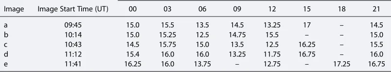
[image:11.612.172.576.126.195.2]From analysis of the UVIS peak auroral brightness along the mapped spacecraft footprint (i.e., at an approximately constant local time of 21 h LT), we see that the oval also moves equatorward from a starting position of 14.5° co-latitude in image (a) to ~16.75° co-latitude by the time of image (e) ~2 h later. This implies that the main auroral emission (and hence associated upward-directedfield-aligned current) is moving equatorward at a rate of ~1.1° per hour (i.e., faster than the Cassini spacecraft equatorward motion quoted above). First, it is interesting to note that the spacecraft remains just poleward of the auroral oval throughout the interval and never maps within the main emission region. This can be seen in Table 1 which shows a comparison between the magnetically mapped spacecraft position in the northern hemisphere and the peak of the main oval brightness along the spacecraft track (i.e., at ~ constant local time of 21 h LT). From Figure 3, and our interpretation of a static current system, we might have expected to see the spacecraft within the auroral emission at the start of the UVIS sequence (i.e., for images a, b, and c), and on the equatorward side of the auroral emission at the times of images d and e. Furthermore, Table 2 shows the co-latitude of the peak brightness of the main auroral emission for eight points in local time around the auroral oval. Importantly, we have used the co-latitude of the equatorward arc (rather than the poleward arc feature) near to 3 h LT, and at 6 h LT where it is clearly visible. Near to midnight, we again refer to the poleward arc rather than the equatorward fainter emission which is not continuously connected (in azimuth) to the emission observed at the magnetically mapped footprint of Cassini near to 21 h LT. Using the data in Table 2, we have performed a simple bestfit analysis to the co-latitude of the peak brightness as a function of local time for each of the images in UVIS sequence considered. The bestfit tilted ellipses in each case are shown as dashed lines in panel (f ) of Figure 4, color coded red, yellow, green, blue, and purple for the images (a)–(e), respectively. The fitted ellipses show that the main emission region indeed moves equatorward near to 21 h LT (seen from the ordering of the colored ellipses (red, yellow, green, blue, and purple) as we move from the pole toward the equator (as indicated by the black arrow). We note, however, that near to 9 h LT, we see the opposite motion as we move from the pole toward the equator, i.e., purple, blue, green, yellow, and red, indicating that the oval is moving poleward at this location (again, as indicated by the black arrow). In addition, we show the
Table 1. Comparison Between the Magnetically Mapped Spacecraft Position in the Northern Hemisphere and the Peak of the Main Oval Brightness Along the Spacecraft Track (i.e., at an Approximately Constant LT of ~21 h), Both Effectively at the Start Time of Each Image
Image Image Start Time (UT) Mapped Spacecraft Footprint (° Co-latitude) Peak Emission (° Co-latitude)
a 09:45 14.1 14.5
b 10:14 14.4 15.0
c 10:43 14.7 15.5
d 11:12 14.9 16.0
center point of the bestfit ellipses using the same color coding which confirms the motion of the auroral oval predominantly toward the 21 h LT sector, with some azimuthal motion evident between images (d) and (e).
However, overall, the UVIS imaging sequence allows us to see that the auroral oval near the magnetically mapped footprint of Cassini at ~21 h LT is not static, but moving equatorward, faster than the spacecraft at a rate of ~1.1° per hour during the ~2 h interval shown here. Finally, we see that on the opposite side of the oval (i.e., near to 09 h LT) the auroral emission is also moving toward the pole. This suggests that the entire oval is tilting (during this relatively short ~2 h interval toward 21 h LT), rather than expanding toward the equator at all local times.
3.3. Interpretation of the Magnetic Field and Auroral Hiss Assuming a Latitudinally Oscillating Current System
We will thus now revisit the in situ data and re-interpret the magneticfield signatures given the above knowledge of a varying relative motion between the spacecraft and the auroralfield-aligned current system. In Figure 5 we show the same 18 h interval on day 4 as shown in Figure 3, but now we show the RPWS frequency time spectrogram in the top panel between 1 Hz and 10 kHz (the auroral hiss frequency range, typically associated with downwardfield-aligned current regions) and the ionospheric Pedersen current (in the same format as Figure 3) in the second panel. Throughout the 18 h interval shown here, we see that the auroral hiss emissions are present from the start, while the spacecraft resides on polar capfield lines. As Cassinifirst encounters thefield-aligned current signatures, we note that the nature of the auroral hiss emission changes significantly, extending to higher frequencies (~1 kHz) and becomes periodic with a short ~1 h modulation present. The auroral hiss emission then“switches off”as the spacecraft crosses through the equatorial plane (as can also be seen in Figure 2). Where the“step-up”in auroral hiss frequency occurs has been defined as a plasmapause-like boundary, which may often be co-located with the open-closed (or related)field line boundary [Gurnett et al., 2010, 2011].
In the third panel we show the cosine of the northern magnetosphere oscillation phase, cos(φN), which is a function of the spacecraft LT [Andrews et al., 2012], while in the bottom panel we show the magnetically mapped ionospheric footprint as before. For reference in thisfinal panel, we now also show the average position of the auroral oval at the local time of the spacecraft footprint (orange) modulated by the northern magnetosphere oscillation phase with maximum amplitude of 2.2°. This amplitude of oscillation is taken from theNichols et al.[2008] study of the HST observations of the southern auroral oval. Marked on with colored dots (using the same color coding as for Figure 4) are the locations of the peak brightness of the oval from UVIS at the start time of each image (as shown in Table 1).
[image:12.612.173.575.128.202.2]We now focus our attention on the northern magnetosphere oscillation phase throughout the interval shown in the third panel. From the work ofProvan et al.[2009b] we know that, as well as tilting the plasma sheet in the equatorial magnetosphere, the perturbation magneticfield associated with the magnetosphere oscillations in the north and in the south acts to tilt the background (internal) magneticfield of Saturn close to the planet in each hemisphere as it rotates. This tilts the auroral oval position toward the equator or the pole as a function of the appropriate hemisphere phase. The northern oval tilts in the same direction as the associated equatorial perturbationfield, while the southern oval tilts away. When cos(φN) = 1, it is expected that the auroral oval would be tilted toward its most equatorward position at the spacecraft LT and,
Table 2. Co-latitude of the Peak Brightness of the Main Auroral Oval for Eight Local Time Values Around the Northern Auroral Ovala
Image Image Start Time (UT)
Peak Emission Latitude (° Co-latitude) as a Function of Local time (h LT)
00 03 06 09 12 15 18 21
a 09:45 15.0 15.5 13.5 14.5 13.25 17 – 14.5
b 10:14 15.0 15.25 12.5 14.75 15.5 – – 15.0
c 10:43 14.5 15.75 15.0 13.5 12.5 16.25 – 15.5
d 11:12 15.4 16.0 16.0 13.25 11.75 16.75 – 16.0
e 11:41 16.25 16.0 13.75 – 12.75 – 17.25 16.75
aThese points are used to derive the bestfit ellipses that are shown in Figure 4f. Where there is no value shown for the
conversely, when the cos(φN) =1, it is expected that the oval will be tilted to its most poleward position. This can be seen in the blue oscillating oval location in the bottom panel. Therefore, as Cassini moves toward the start of thefield-aligned current signatures at ~04:30 UT, we note that the cos(φN) = ~1, and hence we would expect the auroral oval to be tilted toward its most poleward location. At this time, we can see from the ionospheric footprint of Cassini that the spacecraft is moving tangentially to the expected edge of auroral oval (orange) as the oval begins to move equatorward. This would suggest that if the current signature seen here was actually the simple downward/upwardfield-aligned current signature seen in most of the 2008 passes (i.e., Type 1), but that it ismovingequatorward away from the spacecraft (faster than the spacecraft moves equatorward), then the magneticfield/ionospheric Pedersen current signatures are just those of a downwardfield-aligned current region until ~14:00 UT (marked with the downward pointing arrows). At the time of the UVIS image sequence, we see that the spacecraft footprint (in the bottom panel) is poleward of the expected (orange) and actual (multi-colored dots) locations of the main auroral emission as the phase of the northern oscillation acts to tilt the auroral oval toward its most equatorward position, and thus within the
10 10 10 10 10 10 10 10 10
UVIS observation times Field-aligned current regions
RPWS
[image:13.612.222.530.96.472.2]Oscillating current system
poleward auroral-dark downward current region. This interpretation is then consistent with the spacecraft lying near-continuously within the downward current discussed above.
As cos(φN) reaches a maximum, just after the end of the UVIS imaging sequence, the oval at the spacecraft footprint LT begins to move poleward. Now we would expect the mapped spacecraft footprint to cut straight through the expected auroral oval location (orange) before crossing through the equatorial plane shortly afterward. The portion of the ionospheric Pedersen current after the UVIS image sequence then closely resembles the familiar Type 1field-aligned current system reported by [Talboys et al., 2009b], labeled as a downward then upward-directedfield aligned current in Figures 3 and 5. Clearly, the upward-directed portion of thefield-aligned current is directly related to the main oval emission seen near to 21 h LT in the UVIS image sequence, but unfortunately the spacecraft passes across this region just after the end of the UVIS observations, such that we do not have simultaneous image and in situ data at this time. However, we note that according to the simple oscillating oval position depicted in the bottom panel, we would expect that Cassini would pass through the upward current region slightly earlier than it actually did. This is most likely because of the simplicity of the diagram, but may also be associated with an effect of changing auroral oval location associated with (for example) a period of enhanced dayside reconnection, which would then cause the auroral oval to expand to overall larger co-latitudes (see discussion below).
Wefinally note that the RPWS panel at the top of Figure 5 supports the interpretation of the downward-directedfield-aligned current signatures from ~04:30 UT until ~14:15 UT. As discussed above, the auroral hiss emissions are generally thought to be associated with regions of downward-directedfield-aligned current which is certainly supported here. As already noted, we see that the auroral hiss emission is modulated with a 1 h periodicity, and it is interesting to emphasize that this region appears to very closely correlate with the downwardfield-aligned current region shown in the second panel in Figure 5. The origin of the periodicity is currently unknown, but it is often seen in the auroral hiss data and is currently being investigated in other related studies.
4. Discussion and Summary
In this paper we have examined a sequence of multi-instrument data from Rev 99 in January 2009, when the Cassini spacecraft orbit is inclined to the equatorial plane such that views and measurements of thefi eld-aligned currents and related plasma signatures that connect the magnetosphere and the aurora are possible. Previous studies from the 2008 highly inclined orbit phase have shown that thefield-aligned current signatures associated with the main auroral emissions at Saturn appear to have two distinct morphologies. As the spacecraft moves from the pole toward the equator, the spacecraft either encounters a downward/ upwardfield-aligned current structure in the northern and southern hemisphere, or it encounters a downward/upward/downward structure in both cases. These two types, referred to as Type 1 and Type 2, respectively [Talboys et al., 2009b], were seen in approximately 85% of cases in the 2008 data. The other 15% were examples where the type of signature encountered was asymmetric between hemispheres. Why these varying morphologies exist is not clear at present, but it has been suggested that such differences may be related to the magnetosphere oscillation phase.
Analysis of the in situ magneticfield and electron signatures in the interval of interest is presented in Figure 2. By assuming that the current signature is static as a function of time (as the previous analysis byTalboys et al.
[2009a, 2009b, 2011] does, wefind that the data indicate a somewhat differentfield-aligned current structure compared to that described above. With this assumption, we infer a structure made up of four regions, i.e., downward/upward/downward/upward directedfield-aligned currents as the spacecraft moves from the pole toward the equator. The major difference between the geometry of the spacecraft orbit in this interval and those from 2008 is that the spacecraft is further away from the planet near periapsis and thus passes through thefield-aligned current structures much more slowly than in the 2008 data set.
ionospheric footprint of Cassini is consistently poleward of the auroral oval (upward-directedfield-aligned current) throughout the 2 h imaging sequence. Furthermore, analysis of the UVIS images shows that while the auroral oval is moving toward the equator near to 21 h LT, the converse is true on the opposite side of the oval near to 09 h LT. This seems to suggest a tilting motion of the oval toward the 21 h LT sector during this interval, rather than an expansion of the oval toward large co-latitudes at all local times.
When we re-visit the in situ auroral hiss and magneticfield signatures, with knowledge of the motion of the auroral oval, we are able to reinterpret the suggested directions of thefield-aligned current signatures. To aid our interpretation, we also compare the signatures with the northern magnetosphere oscillation phase which we know is associated with the oscillatory motion of the southern auroral oval as observed by HST [Nichols et al., 2008;Provan et al., 2009b]. Throughout this interval, according to the physical picture provided by the
Provan et al.[2009b] analysis, we would expect that during the UVIS interval the auroral oval would be moving equatorward with the spacecraft (which is in agreement with the observations as discussed above). Shortly after the end of the UVIS image sequence, we then expect the oval to have reached its most equatorward position, subsequently moving poleward opposite to the spacecraft motion. Following the UVIS imaging sequence, we indeed see a more familiar Type 1field-aligned current signature, which passes more rapidly across the spacecraft due to the combined effect of the equatorward motion of the spacecraft and the poleward motion of the oval.
Wefind that despite including the oscillatory motion of the auroral oval (upward directedfield-aligned current) when comparing the mapped spacecraft position to the measuredfield-aligned current signatures, the spacecraft actually passes through the upward-directedfield-aligned current somewhat later than expected. We suggest that whilst the magnetosphere oscillation phase is clearly an important factor in modulating the main auroral oval on a large scale, it will not be the only effect. It seems likely that an enhanced episode of dayside reconnection could cause the auroral oval to expand (through the addition of open magneticflux) and is one simple explanation for why the auroral oval is seen slightly later (i.e., at a slightly more equatorward position) than would be expected if the magnetosphere oscillation phase effect was the only factor. Recent studies have shown that reconnection related effects are indeed present in the auroral regions [Radioti et al., 2011;Badman et al.,2012a, 2013], such that the solar wind interaction as a mechanism to modify the auroral oval small- or large-scale features should not be disregarded. It is important to note too that the bright auroral storms observed following solar wind compressions of the magnetosphere have the most dramatic effect on the morphology and brightness of the main auroral oval, causing the auroral oval width to broaden and expand poleward on the dawnside [Clarke et al., 2005, 2009].Cowley et al.
[2005] have proposed that the forward shock at the start of the solar wind compression region triggers an episode of rapid tail reconnection, thus closing open magneticflux in the system and reducing the area of the polar cap. This effect is independent of the magnetosphere oscillation phase effect.
Whether the variable morphology of the Type 1 and Type 2field-aligned current patterns defined byTalboys et al.[2009b], or the netfield-aligned current pattern that emerges from the electron analysis ofSchippers et al.[2012], can be accounted for by the phase of the magnetosphere oscillations remains to be seen, but it certainly seems likely that it is related. However, a further complication may arise due to the presence of the southern hemisphere oscillations in the northern hemisphere (although the converse is not true), which may complicate the details [Provan et al., 2011].
Here we have presented an example case study where we have the crucial combination of in situ observations of thefield-aligned currents, associated plasma signatures, and auroral hiss emission with simultaneous FUV imaging the northern aurora. Wefind that the motion of the auroral oval throughout the imaging sequence is consistent with the appropriate phase of the magnetosphere oscillations in the northern hemisphere at that time. We also deduce that the signature of thefield-aligned currents can be re-interpreted from a static signature to one which has temporal motion, and that the auroral imaging and auroral hiss emissions support that explanation.
References
Andrews, D. J., S. W. H. Cowley, M. K. Dougherty, and G. Provan (2010a), Magneticfield oscillations near the planetary period in Saturn’s equatorial magnetosphere: Variation of amplitude and phase with radial distance and local time,J. Geophys. Res.,115, A04212, doi:10.1029/2009JA014729.
Acknowledgments
EJB, SWHC, and GP are supported by the STFC Leicester Consolidated Grant ST/ K001000/1, and EJB by a Philip Leverhulme Award. SVB is supported by a Royal Astronomical Society Fellowship, and SLJ by an STFC PhD Studentship. DCG is supported by the PRODEX Program managed by the European Space Agency in collabora-tion with the Belgian Federal Science Policy Office. DGM is grateful for the support by the NASA Office of Space Science under Task Order 003 of con-tract NAS5-97271 between NASA Goddard Spaceflight Center and the Johns Hopkins University. The research at the University of Iowa was supported by NASA through contract 1415150 with the Jet Propulsion Laboratory. We thank S Kellock and the Cassini team at Imperial College for MAG data proces-sing, and GR Lewis, N Shane, and LK Gilbert at MSSL for ELS data processing, and acknowledge CS Arridge for useful ELS-related discussions.
Andrews, D. J., A. J. Coates, S. W. H. Cowley, M. K. Dougherty, L. Lamy, G. Provan, and P. Zarka (2010b), Magnetospheric period oscillations at Saturn: Comparison of equatorial and high-latitude magneticfield periods with north and south Saturn kilometric radiation periods,
J. Geophys. Res.,115, A12252, doi:10.1029/2010JA015666.
Andrews, D. J., S. W. H. Cowley, M. K. Dougherty, L. Lamy, G. Provan, and D. J. Southwood (2012), Planetary period oscillations in Saturn’s magnetosphere: Evolution of magnetic oscillation properties from southern summer to post-equinox,J. Geophys. Res.,117, A04224, doi:10.1029/2011JA017444.
Badman, S. V., E. J. Bunce, J. T. Clarke, S. W. H. Cowley, J. C. Gerard, D. Grodent, and S. E. Milan (2005), Openflux estimates in Saturn’s magnetosphere during the January 2004 Cassini-HST campaign, and implications for reconnection rates,J. Geophys. Res.,110, A11216, doi:10.1029/2005JA011240.
Badman, S. V., S. W. H. Cowley, J. C. Gerard, and D. Grodent (2006), A statistical analysis of the location and width of Saturn’s southern auroras,
Ann. Geophys.,24, 3533–3545, doi:10.5194/ANGEO-24-3533-2006.
Badman, S. V., S. W. H. Cowley, L. Lamy, B. Cecconi, and P. Zarka (2008), Relationship between solar wind corotating interaction regions and the phasing and intensity of Saturn kilometric radiation bursts,Ann. Geophys.,26, 3641–3651, doi:10.5194/ANGEO-26-3641-2008. Badman, S. V., et al. (2012a), Rotational modulation and local time dependence of Saturn’s infrared H3
+
auroral intensity,J. Geophys. Res.,117, A09228, doi:10.1029/2012JA017990.
Badman, S. V., et al. (2012b), Cassini observations of ion and electron beams at Saturn and their relationship to infrared auroral arcs,
J. Geophys. Res.,117, A01211, doi:10.1029/2011JA017222.
Badman, S. V., A. Masters, H. Hasegawa, M. Fujimoto, A. Radioti, D. Grodent, N. Sergis, M. K. Dougherty, and A. J. Coates (2013), Bursty magnetic reconnection at Saturn’s magnetopause,Geophys. Res. Lett.,40, 1027–1031, doi:10.1002/grl.50199.
Brandt, P. C., K. K. Khurana, D. G. Mitchell, N. Sergis, K. Dialynas, J. F. Carbary, E. C. Roelof, C. P. Paranicas, S. M. Krimigis, and B. H. Mauk (2010), Saturn’s periodic magneticfield perturbations caused by a rotating partial ring current,Geophys. Res. Lett.,37, L22103, doi:10.1029/ 2010GL045285.
Bunce, E. J. (2012), Origins of Saturn’s auroral emissions and their relationship to large-scale magnetosphere dynamics, inAuroral Phenomenology and Magnetospheric Processes: Earth and Other Planets,Geophys. Monogr. Ser., vol. 197, edited by A. Keiling et al., pp. 397–410, AGU, Washington, D. C., doi:10.1029/2011GM001191.
Bunce, E. J., S. W. H. Cowley, D. M. Wright, A. J. Coates, M. K. Dougherty, N. Krupp, W. S. Kurth, and A. M. Rymer (2005), In situ observations of a solar wind compression-induced hot plasma injection in Saturn’s tail,Geophys. Res. Lett.,32, L20S04, doi:10.1029/2005GL022888. Bunce, E. J., S. W. H. Cowley, C. M. Jackman, J. T. Clarke, F. J. Crary, and M. K. Dougherty (2006), Cassini observations of the Interplanetary
Medium Upstream of Saturn and their relation to the Hubble Space Telescope aurora data,Adv. Space Res.,38, 806–814, doi:10.1016/J. ASR.2005.08.005.
Bunce, E. J., S. W. H. Cowley, I. I. Alexeev, C. S. Arridge, M. K. Dougherty, J. D. Nichols, and C. T. Russell (2007), Cassini observations of the variation of Saturn’s ring current parameters with system size,J. Geophys. Res.,112, A10202, doi:10.1029/2007JA012275.
Bunce, E. J., et al. (2008), Origin of Saturn’s aurora: Simultaneous observations by Cassini and the Hubble Space Telescope,J. Geophys. Res.,
113, A09209, doi:10.1029/2008JA013257.
Carbary, J. F. (2012), The morphology of Saturn’s ultraviolet aurora,J. Geophys. Res.,117, A06210, doi:10.1029/2012JA017670. Carbary, J. F. (2013), Longitude dependences of Saturn’s ultraviolet aurora,Geophys. Res. Lett.,40, 1902–1906, doi:10.1002/grl.50430. Clarke, J. T., et al. (2005), Morphological differences between Saturn’s ultraviolet aurorae and those of Earth and Jupiter,Nature,433, 717–719,
doi:10.1038/NATURE03331.
Clarke, J. T., et al. (2009), Response of Jupiter’s and Saturn’s auroral activity to the solar wind,J. Geophys. Res.,114, A05210, doi:10.1029/ 2008JA013694.
Cowley, S. W. H., E. J. Bunce, and J. M. O’Rourke (2004a), A simple quantitative model of plasmaflows and currents in Saturn’s polar ionosphere,
J. Geophys. Res.,109, A05212, doi:10.1029/2003JA010375.
Cowley, S. W. H., E. J. Bunce, and R. Prange (2004b), Saturn’s polar ionosphericflows and their relation to the main auroral oval,Ann. Geophys.,
22, 1379–1394, doi:10.1029/2003JA010375.
Cowley, S. W. H., S. V. Badman, E. J. Bunce, J. T. Clarke, J. C. Gerard, D. Grodent, C. M. Jackman, S. E. Milan, and T. K. Yeoman (2005), Reconnection in a rotation-dominated magnetosphere and its relation to Saturn’s auroral dynamics,J. Geophys. Res.,110, A02201, doi:10.1029/2004JA010796.
Cowley, S. W. H., C. S. Arridge, E. J. Bunce, J. T. Clarke, A. J. Coates, M. K. Dougherty, J. C. Gerard, D. Grodent, J. D. Nichols, and D. L. Talboys (2008), Auroral current systems in Saturn’s magnetosphere: comparison of theoretical models with Cassini and HST observations,Ann. Geophys.,26, 2613–2630, doi:10.5194/ANGEO-26-2613-2008.
Crary, F. J., et al. (2005), Solar wind dynamic pressure and electricfield as the main factors controlling Saturn’s aurorae,Nature,433, 720–722, doi:10.1038/NATURE03333.
Dougherty, M. K., et al. (2004), The Cassini magneticfield investigation,Space Sci. Rev.,114, 331–383, doi:10.1007/S11214-004-1432-2. Dougherty, M. K., et al. (2005), Cassini magnetometer observations during Saturn orbit insertion,Science,307, 1266–1270, doi:10.1126/
SCIENCE.1106098.
Grodent, D., J. C. Gérard, S. W. H. Cowley, E. J. Bunce, and J. T. Clarke (2005), Variable morphology of Saturn’s southern ultraviolet aurora,
J. Geophys. Res.,110, A07215, doi:10.1029/2004JA010983.
Grodent, D., A. Radioti, B. Bonfond, and J.-C. Gérard (2010), On the origin of Saturn’s outer auroral emission,J. Geophys. Res.,115, A08219, doi:10.1029/2009JA014901.
Grodent, D., J. Gustin, J.-C. Gérard, A. Radioti, B. Bonfond, and W. R. Pryor (2011), Small-scale structures in Saturn’s ultraviolet aurora,
J. Geophys. Res.,116, A09225, doi:10.1029/2011JA016818.
Gurnett, D. A., A. Lecacheux, W. S. Kurth, A. M. Persoon, J. B. Groene, L. Lamy, P. Zarka, and J. F. Carbary (2009a), Discovery of a north-south asymmetry in Saturn’s radio rotation period,Geophys. Res. Lett.,36, L16102, doi:10.1029/2009GL039621.
Gurnett, D. A., A. M. Persoon, J. B. Groene, A. J. Kopf, G. B. Hospodarsky, and W. S. Kurth (2009b), A north-south difference in the rotation rate of auroral hiss at Saturn, Comparison to Saturn’s kilometric radio emission,Geophys. Res. Lett.,36, L21108, doi:10.1029/ 2009GL040774.
Gurnett, D. A., et al. (2004), The Cassini Radio and Plasma Wave investigation,Space Sci. Rev.,114, 395–463, doi:10.1007/S11214-004-1434-0. Gurnett, D. A., et al. (2010), A plasmapause-like density boundary at high latitudes in Saturn’s magnetosphere,Geophys. Res. Lett.,37, L16806,
doi:10.1029/2010GL044466.
Gurnett, D. A., A. M. Persoon, J. B. Groene, W. S. Kurth, M. Morooka, J.-E. Wahlund, and J. D. Nichols (2011), The rotation of the plasmapause-like boundary at high latitudes in Saturn’s magnetosphere and its relation to the eccentric rotation of the northern and southern auroral ovals,
Gustin, J., B. Bonfond, D. Grodent, and J.-C. Gérard (2012), Conversion from HST ACS and STIS auroral counts into brightness, precipitated power, and radiated power for H2giant planets,J. Geophys. Res.,117, A07316, doi:10.1029/2012JA017607.
Jackman, C. M., N. Achilleos, E. J. Bunce, S. W. H. Cowley, M. K. Dougherty, G. H. Jones, S. E. Milan, and E. J. Smith (2004), Interplanetary magneticfield at ~ 9 AU during the declining phase of the solar cycle and its implications for Saturn’s magnetospheric dynamics,
J. Geophys. Res.,109, A11203, doi:10.1029/2004JA010614.
Jackman, C. M., N. Achilleos, S. W. H. Cowley, E. J. Bunce, A. Radioti, D. Grodent, S. V. Badman, M. K. Dougherty, and W. Pryor (2013), Auroral counterpart of magneticfield dipolarizations in Saturn’s tail,Planet. Space Sci.,82-83, 34–42, doi:10.1016/J.PSS.2013.03.010.
Kanani, S. J., et al. (2010), A new form of Saturn’s magnetopause using a dynamic pressure balance model, based on in situ, multi-instrument Cassini measurements,J. Geophys. Res.,115, A06207, doi:10.1029/2009JA014262.
Kellett, S., E. J. Bunce, S. W. H. Cowley, and A. J. Coates (2009), Thickness of Saturn’s ring current determined from north-south Cassini passes through the current layer,J. Geophys. Res.,114, A04209, doi:10.1029/2008JA013942.
Kopf, A. J., et al. (2010), Electron beams as the source of whistler-mode auroral hiss at Saturn,Geophys. Res. Lett.,37, L09102, doi:10.1029/ 2010GL042980.
Kurth, W. S., et al. (2005), An Earth-like correspondence between Saturn’s auroral features and radio emission,Nature,433, 722–725, doi:10.1038/NATURE03334.
Lamy, L., B. Cecconi, R. Prangé, P. Zarka, J. D. Nichols, and J. T. Clarke (2009), An auroral oval at the footprint of Saturn’s kilometric radio sources, colocated with the UV aurorae,J. Geophys. Res.,114, A10212, doi:10.1029/2009JA014401.
Lamy, L., R. Prangé, W. Pryor, J. Gustin, S. V. Badman, H. Melin, T. Stallard, D. G. Mitchell, and P. C. Brandt (2013), Multispectral simultaneous diagnosis of Saturn’s aurorae throughout a planetary rotation,J. Geophys. Res. Space Physics,118, 4817–4843, doi:10.1002/jgra.50404. Milan, S. E., M. Lester, S. W. H. Cowley, K. Oksavik, M. Brittnacher, R. A. Greenwald, G. Sofko, and J.-P. Villain (2003), Variations in polar cap area
during two substorm cycles,Ann. Geophys.,21, 1121–1140, doi:10.5194/ANGEO-21-1121-2003.
Mitchell, D. G., S. M. Krimigis, C. Paranicas, P. C. Brandt, J. F. Carbary, E. C. Roelof, W. S. Kurth, D. A. Gurnett, J. T. Clarke, and J. D. Nichols (2009a), Recurrent energization of plasma in the midnight-to-dawn quadrant of Saturn’s magnetosphere, and its relationship to auroral UV and radio emissions,Planet. Space Sci.,57, 1732–1742, doi:10.1016/J.PSS.2009.04.002.
Mitchell, D. G., W. S. Kurth, G. B. Hospodarsky, N. Krupp, J. Saur, B. H. Mauk, J. F. Carbary, S. M. Krimigis, M. K. Dougherty, and D. C. Hamilton (2009b), Ion conics and electron beams associated with auroral processes on Saturn,J. Geophys. Res.,114, A02212, doi:10.1029/ 2008JA013621.
Nichols, J. D., J. T. Clarke, S. W. H. Cowley, J. Duval, A. J. Farmer, J. C. Gérard, D. Grodent, and S. Wannawichian (2008), Oscillation of Saturn’s southern auroral oval,J. Geophys. Res.,113, A11205, doi:10.1029/2008JA013444.
Prange, R., L. Pallier, K. C. Hansen, R. Howard, A. Vourlidas, G. Courtin, and C. Parkinson (2004), An interplanetary shock traced by planetary auroral storms from the Sun to Saturn,Nature,432, 78–81, doi:10.1038/nature02986.
Provan, G., D. J. Andrews, C. S. Arridge, A. J. Coates, S. W. H. Cowley, S. E. Milan, M. K. Dougherty, and D. M. Wright (2009a), Polarization and phase of planetary-period magneticfield oscillations on high-latitudefield lines in Saturn’s magnetosphere,J. Geophys. Res.,114, A02225, doi:10.1029/2008JA013782.
Provan, G., S. W. H. Cowley, and J. D. Nichols (2009b), Phase relation of oscillations near the planetary period of Saturn’s auroral oval and the equatorial magnetospheric magneticfield,J. Geophys. Res.,114, A04205, doi:10.1029/2008JA013988.
Provan, G., D. J. Andrews, B. Cecconi, S. W. H. Cowley, M. K. Dougherty, L. Lamy, and P. M. Zarka (2011), Magnetospheric period magneticfield oscillations at Saturn: Equatorial phase "jitter" produced by superposition of southern and northern period oscillations,J. Geophys. Res.,
116, A04225, doi:10.1029/2010JA016213.
Radioti, A., D. Grodent, J. C. Gerard, E. Roussos, C. Paranicas, B. Bonfond, D. G. Mitchell, N. Krupp, S. Krimigis, and J. T. Clarke (2009), Transient auroral features at Saturn: Signatures of energetic particle injections in the magnetosphere,J. Geophys. Res.,114, A03210, doi:10.1029/ 2008JA013632.
Radioti, A., D. Grodent, J. C. Gerard, S. E. Milan, B. Bonfond, J. Gustin, and W. Pryor (2011), Bifurcations of the main auroral ring at Saturn: ionospheric signatures of consecutive reconnection events at the magnetopause,J. Geophys. Res.,116, A11209, doi:10.1029/ 2011JA016661.
Schippers, P., et al. (2008), Multi-instrument analysis of electron populations in Saturn’s magnetosphere,J. Geophys. Res.,113, A07208, doi:10.1029/2008JA013098.
Schippers, P., N. André, D. A. Gurnett, G. R. Lewis, A. M. Persoon, and A. J. Coates (2012), Identification of the electronfield-aligned current systems in Saturn’s magnetosphere,J. Geophys. Res.,117, A05204, doi:10.1029/2011JA017352.
Talboys, D. L., C. S. Arridge, E. J. Bunce, A. J. Coates, S. W. H. Cowley, and M. K. Dougherty (2009a), Characterization of auroral current systems in Saturn’s magnetosphere: High-latitude Cassini observations,J. Geophys. Res.,114, A06220, doi:10.1029/2008JA013846.
Talboys, D. L., C. S. Arridge, E. J. Bunce, A. J. Coates, S. W. H. Cowley, M. K. Dougherty, and K. K. Khurana (2009b), Signatures offield-aligned currents in Saturn’s nightside magnetosphere,Geophys. Res. Lett.,36, L19107, doi:10.1029/2009GL039867.
Talboys, D. L., E. J. Bunce, S. W. H. Cowley, C. S. Arridge, A. J. Coates, and M. K. Dougherty (2011), Statistical characteristics offield-aligned currents in Saturn’s nightside magnetosphere,J. Geophys. Res.,116, A04213, doi:10.1029/2010JA016102.