Computational Analysis of Tumor Angiogenesis Patterns Using a Two dimensional Model

Vol. 46, No. 2, pp. 275 - 283, 2005

Tumor angiogenesis was simulated using a two-dimensional computational model. The equation that governed angiogenesis comprised a tumor angiogenesis factor (TAF) conservation equation in time and space, which was solved numerically using the Galerkin finite element method. The time derivative in the equation was approximated by a forward Euler scheme. A stochastic process model was used to simulate vessel formation and vessel elongation towards a paracrine site, i.e., tumor-secreted basic fibroblast growth factor (bFGF). In this study, we assumed a two-dimensional model that represented a thin (1.0 mm) slice of the tumor. The growth of the tumor over time was modeled according to the dynamic value of bFGF secreted within the tumor. The data used for the model were based on a previously reported model of a brain tumor in which four distinct stages (multicellular spherical, first detectable lesion, diagnosis, and death of the virtual patient) were modeled. In our study, computation was not continued beyond the 'diagnosis' time point to avoid the computational complexity of analyzing numerous vascular branches. The numerical solutions revealed that no bFGF remained within the region in which vessels developed, owing to the uptake of bFGF by endothelial cells. Consequently, a sharp declining gradient of bFGF existed near the surface of the tumor. The vascular architecture developed numerous branches close to the tumor surface (the brush-border effect). Asymmetrical tumor growth was associated with a greater degree of branching at the tumor surface.

Key Words: Tumor growth, angiogenesis, computational modeling, basic fibroblast growth factor

INTRODUCTION

Despite substantial progress in therapeutic efforts, the outcome of some malignant cancers re-mains very poor. Novel therapies are being devel-oped, one of which is a method to suppress cancer angiogenesis that was proposed by Folkman1 _and others.

There have been many modeling studies of tumor angiogenesis in which continuous or dis-crete models were used. In continuous models, only the distribution of enthothelial cells is considered; vascular networks are not included. Chaplain et al.2,3presented two- and three-dimen-sional models of tumor angiogenesis using a combination of both the discrete and continuous method. To determine the movement of the sprouting tips of enthothelial cells, the authors solved partial differential equations of the concen-tration of a tumor angiogenesis factor (TAF), fibronectin concentrations, and endothelial cell density using the finite difference method. The formation and growth of vessel sprouts were approximated using a stochastic process that was based on the distribution of TAF and fibronectin. Chaplain et al.2,3also assumed that TAF secretion was constant over time. The numerical solutions of such models can be compared to experimental data, and cellular mechanisms can be incor-porated readily into new mathematical models. Lastly, Gazit et al.4 _{used fractal theory to compute} the vessel networks that surrounded a tumor and computed the hemodynamics within the vessel structures.

Computational Analysis of Tumor Angiogenesis Patterns

Using a Two-dimensional Model

Eun Bo Shim1, Young-Guen Kwon2, and Hyung Jong Ko3

1_{Department of Mechanical & Biomedical Engineering, Kangwon National University, Chunchon, Kangwon-do, Republic of}

Korea;

2_{Department of Biochemistry, Yonsei University, Seoul, Republic of Korea;}

3_{Department of Mechanical Engineering, Kumoh National Institute of Technology, Kumi, Kyungbuk, Republic of Korea.}

Received September 8, 2004 Accepted November 18, 2004

This work was supported by the Korea Research Foundation Grant. (KRF-2003-002-D00399)

C L u C k y C x C D t C 2 2 2 2 × × -× -÷÷ ø ö çç è æ ¶ ¶ + ¶ ¶ × = ¶ ¶

{

}

0 0 C C

f (C)

1 exp (C C ) C C

£ < ì

= í _{- -a - £}

î

MATERIALS AND METHODS

Previous works

Recently, Tong et al.5 _{developed a} two-dimen-sional model of angiogenesis in which they assumed a biased random motion of endothelial cells. To obtain basic information about the biased growth of endothelial cells, the authors examined the transport of angiogenic factors in rat cornea. Because vessel growth in their study was independent of the computation mesh (unlike Chaplain's model), tumor angiogenesis was implemented in a more realistic and efficient manner. However, one of the main problems with previous models is that the quantity of angiogenic factors that are released from tumor cells is assumed to be constant. This assumption is unrealistic because as the volume of a tumor increases, the quantity of angiogenic factors that are released also increases.

In the present study, we present a computatio-nal model of tumor-induced angiogenesis for a growing brain tumor, based on Tong's model.5 However, in contrast to Tong's and other models, our model includes dynamic (time-varying) release of angiogenic factors from tumor cells. The model of the growing brain tumor that we used was adopted from the work of Kansal et al.6 The quantity of TAF released from a growing brain tumor depends on the volume of the tumor and the number of constituent cells. We selected basic fibroblast growth factor (bFGF) as a TAF, because the concentration of bFGF is reportedly proportional to the increase in malig-nancy and vascularity of high-grade gliomas.7,8 Some parameter values for bFGF-induced angio-genesis were obtained from Tong et al.,6 _{and we} used 50 pg/105 _{cells per 24 h as the production} rate for bFGF by human U87 glioma cells.9 _The finite element method was used to solve the convection-diffusion equation for the concentra-tion of bFGF. This method is a convenient way with which to deal with the complex geometry of real biological phenomena. Both vessel forma-tion and sprout elongaforma-tion were simulated using a stochastic process as in the aforementioned studies.

Model

Algorithm

Transport equation for basic fibroblast growth factor The transport of bFGF within tissue depends on the diffusion of this molecule into the interstitial space, uptake of bFGF by endothelial cells, and chemical inactivation of bFGF within the extracel-lular space. The partial differential equation of bFGF transport is represented in Eq. (1), which was obtained from Tong et al.5

(1)

In Eq. (1), C, D, k, u, and L represent the concentration of bFGF, the diffusion coefficient of bFGF, the rate constant of bFGF degradation, the rate constant of bFGF uptake, and vessel density (defined as the total vessel length per unit area), respectively. For the computational domain, application of the Galerkin finite element dis-cretization for Eq. (1) yielded the following matrix equation.

KX=R (2)

In this matrix, K is the stiffness matrix, X is the vector of unknown nodal variables of C, and R contains the external driving forces. The matrix Eq. (2) was solved using an incomplete conjugate gradient method.10

Sprout formation and elongation

The initial response of the endothelial cells to bFGF is chemotactic, and this initiates the migra-tion of endothelial cells towards the bFGF-re-leasing tumor. Thereafter, small capillary sprouts are formed. The sprouts increase in length owing to the migration and recruitment of endothelial cells. The sprouts continue to grow towards the growing tumor, guided by the motion of the leading endothelial cell at the tip of the sprout. First, we introduced a threshold function f(C) to account for the effect of concentration of bFGF on sprout formation and elongation, as follows.

t l ) C ( f S

n= max D D

(

)

0 1 exp( Bt) B

A exp R R

þ ý ü î

í ì

÷ ø ö ç

è

æ _-

-=

In Eq. (3), Ct is the threshold concentration and

αis a constant that controls the shape of the curve.

To approximate sprout formation, we assumed it to be a stochastic process. The probability n⁻ for the formation of one sprout from a vessel segment in a time interval between t and t+ t is pro-portional to t, the segment length l, and the threshold function, as follows:

(4)

In Eq. (4), Smax is a rate constant that deter-mines the maximum probability of sprout forma-tion per unit time and vessel length.

The growth of a sprout is determined by the locomotion of its tip, while the geometry of a sprout depends on the tip trajectory.10 The direction of sprout growth at each time step depends on two unit vectors: the direction of growth in the previous time step and the direction of the concentration gradient of the angiogenic factors. This is because sprout growth depends on endothelial cell migration, which has a tendency to persist in the same direction as in the previous time step. To reflect the effect of the extracellular matrix on cell migration, we assumed that the angle of deviation, , was between 90 and -90θ

and that tan had a Gaussian distribution with a mean of zero and a variance of σ2_{. A detailed}

description of sprout formation and elongation can be found in the reference.5

Brain tumor growth model

We used a model of a brain tumor that had four distinct growth stages, namely spherical, detec-table lesion, diagnosis, and death.6 _To approxi-mate data in each of these growth stages, we used the following Gompertz equation:

(5)

In Eq. (5), A and B are parameters and is the initial volume. The quantity of bFGF release at each of the four stages is summarized in Table 2. We assumed that tumor growth was spherical and investigated a 1.0-mm-thick, circular slice of the tumor for our two-dimensional model. As both the proliferative and quiescent tumor cell fractions likely release bFGF, we calculated the amount of bFGF at each of the four stages for the total amount of living tumor cells using the cell numbers reported by Kansal et al.6

Analysis

Two-dimensional simulation model

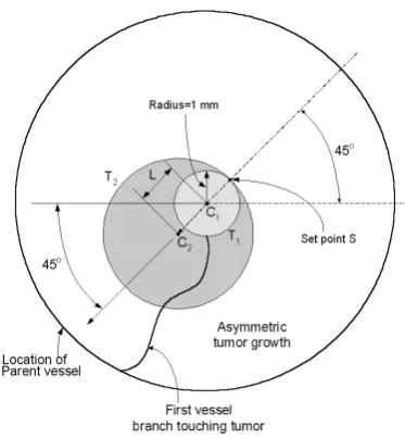
The two-dimensional model is depicted in Fig. 1. In Fig. 1, Ldomain, RPV and Rt represent the distribution of bFGF, the radius of the parent vessel measured from the center of the tumor, and the tumor radius, respectively. We assumed that the radius of the tumor increased over time and calculated the tumor radius using Eq. (6).

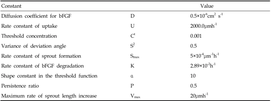
Table 1. Values of Model Constants for the Standard Case of Tumor Growth

Constant Value

Diffusion coefficient for bFGF D 0.5×10-6_cm2 _s-1 Rate constant of uptake U 2000.0 mhμ -1

Threshold concentration Ct _0.001 Variance of deviation angle S2 _0.5

Rate constant of sprout formation Smax 5×10-4μm-1h-1 Rate constant of bFGF degradation K 2.89×10-2_h-1 Shape constant in the threshold function α 10

Persistence ratio P 0.5

(

)÷

è

æ _-

-= 1 exp( Bt) B

A exp V

V 0 (6)

In Eq. (6), R0 was assumed to be 1.0 mm as an initial condition. RPV was selected to allow the first branch to reach the source at a time point at which the tumor radius was 1.0 mm.11 We found that a lattice disk with a radius of 4.5 mm satisfied this condition, and Ldomain was assumed to cover the disc. We also assumed that bFGF was released continually from the tumor, which was located at the center of the aforementioned disk (i.e., repre-sented as a solid circle in a transverse section of the tumor). The region into which angiogenic factors diffused was a 10.0×10.0-mm square (Ldomain=10.0 mm). Three points of initial sprouting were located between 180 and 270 .

Initial and boundary conditions

To solve the equation that governed the concentrations of angiogenic factors (Eq. (1)), a 'no flux' condition was assumed for bFGF transport at the boundary of the diffusion region. The initial

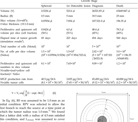
Table 2. Approximate Concentration of Basic Fibroblast Growth Factor (bFGF) Released during Each of the Four Consecutive Growth Stages Used to Simulate Growth of a Brain Tumor (based on Ref. 6).

Growth Stage

Spheroid 1st Detectable lesion Diagnosis Death Volume (V) 0.5236μl 523.6μl 26521.85μl 65449.847μl Radius (R) 0.5 mm 5 mm 18.5 mm 25 mm Slice volume (Vs= Rπ 2t)

t=slice thickness (=0.1.0 mm) 0.07854μl 7.854μl 107.521.0μl 196.35μl

Proliferative and quiescent cell volume per slice (cell fraction)

0.0424μl (54%)

4.0μl (51%)

48.4μl (45%)

78.5μl (40%) Elapsed time of tumor growth

(simulation results6₎ 69 days 223 days 454 days 560 days Total number of cells (Ntotal) 106 ₁₀9 _{5 × 10}10 ₁₀11 No. of cells per slice volume

(Nslice)

1.5 × 105

(106_{× 0.07854/0.5236)} 1.5×10 7

(109_{×7.854/523.6)} 2.02 × 10 8

(5 × 1010_{× 107.521} /26521.8)

3.0 × 108 (1011_{× 196.35} /65449.85) Proliferative and quiescent cell

numbers in slice volume Nviable=(red+yellow cell fraction)× Nslice

8.1 × 104 _7.65×106 _{9.09 × 10}7 _{1.2 × 10}8

bFGF production rate from Nviable tumor cells

40.5 pg/24 h

(8.1 × 104_{× 50/10}5₎ 3,825 pg/24 h_{(7.65 × 10}6_{× 50/10}5₎ 45,450 pg/24 h_{(9.12 × 10}7_{× 50/10}5₎ 60,000 pg/24 h_{(1.2 × 10}8_{× 50/10}5₎

concentration of bFGF was zero within the com-putational region. For comcom-putational convenience, we assumed that the initial radius of the tumor was 0.1 mm. The concentration of bFGF at the tumor site increased with the tumor volume, which concurs with a cellular automaton model described previously, in which a growing brain tumor was simulated over several orders of magnitude.6 Table 2 shows the rate of bFGF production over time. For the space discretization of the computational domain, a 200 × 200 finite element lattice was used and linear approxima-tions of the variables within elements were assumed. We calculated both symmetrical and asymmetrical tumor growth.

For asymmetrical tumor growth, we assumed that tumor growth was symmetrical before the first vessel branch made contact with the tumor surface; thereafter, growth was assumed to be asymmetrical (see Eq. (7)). As represented in Fig. 2, the vessel branch contacted the tumor surface when R=1.0 mm (T1 tumor with center point C1), after which the tumor began to grow eccentrically. The eccentricity L at time t (T2 tumor with center point C2) owing to asymmetrical tumor growth was defined as follows:

L=(t-tref)Vecc if t > tref (7)

In Eq. (7), t and tref represent the arbitrary time

and reference time at which the first vessel branch made contact with the tumor surface, respectively. According to the preliminary computation, tref was -2,600 h. Vecc is a variable that represents the rate of eccentricity change; therefore, the eccentric distance at a time t can be expressed as Eq. (7). In this study, we assumed that Vecc=0.003 mm/h. The direction of eccentricity was 225 . In the equa-tion above, note that only the part of the tumor that was facing the blood vessels grew.

Branching pattern analysis

To quantify the vessel branching pattern within the computational domain, we calculated the number of branching points within a given region of interest (ROI). A ROI was defined as 50 circular areas that divided the space between the central tumor domain and the circle from which the parent vessel originated (see Fig. 1). A branching point was defined as the site at which one vessel was divided into two new vessels (Fig. 1). For each ROI, the total number of branching points within the ROI was calculated according to the average distance of the ROI from the parent vessel. To take into account temporal variation of vessel growth, we considered the total length of vessels at certain time points (equivalent to the sum of the lengths of all vessels that existed at that point in time).

RESULTS

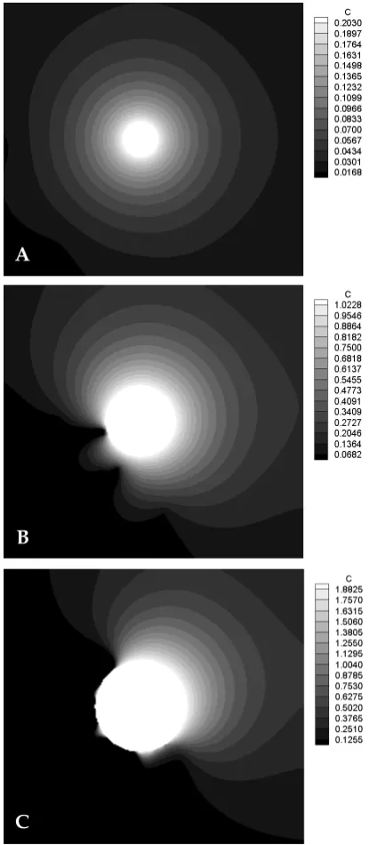
First, we computed a standard case for the parameters as shown in Table 1. Dynamic changes in the tumor radius and the concentration of bFGF (Fig. 3) were computed from Eq. (6). Compared to the tumor radius, the concentration of bFGF had a sharper gradient after t=3,000 h. The concentra-tion distribuconcentra-tion over time of bFGF (Fig. 4) re-vealed that the concentration distribution of bFGF was a radial isotropic gradient at t=1,656 h (spherical state), because the bFGF excreted from the tumor diffused spatially in all directions and only very short branches existed close to the par-ent vessel. As the branched vessels grew toward the tumor surface, bFGF consumption occurred around these vessels. The radial gradient of the concentration distribution of bFGF ceased to vary isotropically; the concentration of bFGF was very Fig. 2. Two-dimensional model geometry for

low on the side on which the vessels were growing and was relatively high on the side op-posite to the parent vessel (Fig. 4(B) and (C)).

The vessel branching pattern for symmetrical tumor growth is shown in Fig. 5. Initially, three branches from the parent vessel grew toward the tumor following the concentration gradient of bFGF. The lowest branch appeared to be very short initially, but subsequently branched numer-ous times as it approached the tumor surface. In our simulation, the first vessel branch touched the tumor surface at t=2,590 h; this vessel branching pattern is exemplified by the pattern in Fig. 5(B), which illustrates the branching pattern at t=2,600 h. At t=3,200 h, there were numerous vessel branches close to the tumor surface (the brush-border effect; Fig. 5(C)).

The pattern of vessel growth for symmetrical tumor growth is illustrated in Fig. 6. At t=1565 and t=2600 h, the number of branching points near the tumor surface was largely unchanged, whereas at t=2800 and t=3000 h, there was a marked increase in the number of branching points near the tumor surface. The total vessel length was relatively constant initially, but in-creased sharply after the first vessel reached the tumor surface at t=2,590 h (Fig. 7).

Asymmetrical tumor growth is illustrated in Fig. 8 and 9. Unlike symmetrical tumor growth, asymmetrical growth was associated with slightly elevated concentrations of bFGF at the tumor

sur-face (Fig. 8), which acted as promoter that en-hanced branching of the parent vessel. Never-theless, the difference in the concentration of bFGF during symmetrical and asymmetrical growth was small. Fig. 9 illustrates that asym-metrical tumor growth was biased toward the Fig. 3. Radius of the tumor and concentration of basic

fibroblast growth factor (bFGF) over time.

Fig. 4. Contours of concentration gradient for bFGF (relative to bFGF concentration for a tumor radius of 1.0 mm at t=2,590 h) over time for the standard case of sym-metrical tumor growth. (A) t=1,656 h (spherical growth stage). (B) t=2,600 h. (C) t=3,000 h.

A

B

parent vessel. Although the pattern of vessel branching was similar to the case of symmetrical growth, branches generated from the lowest location of the parent vessel during asymmetrical

growth were more densely distributed close to the tumor surface as compared to during symmetrical growth. Changes in the total vessel length during asymmetrical tumor growth were similar to those that occurred during symmetrical growth, but the total vessel length was slightly greater after t= 3,000 h as compared to that during symmetrical growth.

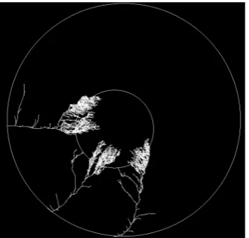
Fig. 5. Vessel structures over time for the standard case of symmetrical growth (Smax=0.5). (A) t=1,656 h (spherical growth stage). (B) t=2,600 h. (C) t=3,200 h.

Fig. 6. Number of branching points versus the ROI, i.e., the radial distance between the parent vessel and the tumor surface.

Fig. 7.Total vessel length over time for the standard case of symmetrical tumor growth.

A

B

DISCUSSION

In this study we proposed a new computational method to simulate tumor angiogenesis in two dimensions. For the analysis of the spatial distri-bution of bFGF over time, the bFGF conservation equation was solved using a finite element method. Unlike previous studies, we assumed that the tumor grew over time in our model. This allowed us to observe the effect of dynamic bFGF production and its effect on vessel branching patterns. The brain tumor model proposed by Kansal et al.6 _{was used as a basis for our model}

of a growing tumor, which comprised four dis-tinct stages, namely spherical state, first detectable lesion, diagnosis, and death. In the present study, we computed both symmetrical and asymmetrical tumor growth and compared the results of each. Biased tumor growth toward vessel branches was assumed to simulate the asymmetric growth of the tumor.

From a computational aspect, we used a finite element method to solve the conservation equa-tion of bFGF concentraequa-tions, whereas a finite difference method was used in previous studies. It is widely recognized that the finite element method is more flexible when dealing with com-plex geometry. In addition, it is relatively easy to implement boundary conditions with this method. However, the finite element method requires more computing time than the finite difference method. If a realistic tumor geometry obtained from magnetic resonance imaging data is adopted as the computational model, the finite element method is better suited to solving the equations for such a complex shape. If the finite element method that we used is combined with an auto-matic mesh generation program in a two-dimen-sional (triangular mesh) or three-dimentwo-dimen-sional (tet-rahedron mesh) geometry, a realistic (and there-fore clinically relevant) tumor can be simulated. Our model is novel in that we simulated a tumor that grew and exhibited angiogenic re-sponses to changing concentrations of bFGF. As shown in Fig. 7, the number of vessel branches increased dramatically as soon as a vessel branch made contact with the tumor surface for the first time. This can be explained physiologically by the fact that tumors generally grow rapidly once blood is supplied to them directly from a parent vessel; therefore, tumors exhibit a bias in growth that is skewed towards the parent vessel. To examine the effect on angiogenesis of such biased tumor growth, we computed a comparison of asymmetrical and symmetrical tumor growth. In the case of symmetrical growth, bFGF was almost completely consumed at the tumor surface. By contrast, there were slightly higher concentrations of bFGF at the tumor surface during asymmetrical growth, which acted as a promoter that enhanced the branching of the parent vessel.

Fig. 8. Contours of concentration gradient for bFGF (relative to bFGF concentration for a tumor radius of 1.0 mm at t=2,590 h) at t=3,000 h for asymmetrical growth.

REFERENCES

1. Folkman J. Angiogenesis in cancer, vascular, rheuma-toid and other disease. Nature Med 1995;1:21-31. 2. Chaplain MAJ. Avascular growth, angiogenesis and

vascular growth in solid tumours: the mathematical modelling of the stages of tumour development. Math Comput Model 1996;23:47-87.

3. Chaplain MAJ, Anderson ARA. The mathematical modelling, simulation and prediction of tumour-in-duced angiogenesis. Invasion Metastasis 1997;16:222-34. 4. Gazit Y, Berk DA, Leunig M, Baxter LT, Jain RK. Scale-invariant behavior and vascular network forma-tion in normal and tumor tissue. Phys Rev Lett 1995; 75:2428-31.

5. Tong S, Yuan F. Numerical simulations of angiogenesis in the cornea. Microvasc Res 2001;61:14-27.

6. Kansal AR, Torquato S, Harsh GR, Chiocca EA, Deisboeck TS. Simulated brain tumor growth dynamics using a three-dimensional cellular automation. J Theor Biol 2000;203:1-18.

7. Takahashi JA, Fukumuto M, Igarashi K, Oda Y, Kikuchi H, Hatanaka M. Correlation of basic fibroblast growth factor expression levels with the degree of malignancy and vascularity in human gliomas. J Neurosurg 1992; 76:792-8.

8. Zagzag D, Miller DC, Sato Y, Rifkin DB, Burstein DE. Immunohistochemical localization of basic fibroblast growth factor in astrocytomas. Cancer Res 1990;50:7393-8.

9. Sato Y, Murphy PR, Sato R, Friesen HG. Fibroblast growth factor release by bovine endothelial cells and human astrocytoma cells in culture is density depen-dent. Mol Endocrinol 1989;3:744-8.

10. Kershaw D. The incomplete Cholesky-conjugate gradi-ent method for the iterative solution of linear equa-tions. J Comput Phys 1978;26:43-65.