Citation:
Subbiah, U and Ramachandran, M and Mahmood, Z (2019) Software engineering approach to bug prediction models using machine learning as a service (MLaaS). In: ICSOFT 2018 - 13th International Conference on Software Technologies, 26th to 28th July 2018, Porto, Portugal.
Link to Leeds Beckett Repository record: http://eprints.leedsbeckett.ac.uk/6191/
Document Version:
Conference or Workshop Item
Creative Commons: Attribution-Noncommercial-No Derivative Works 4.0
Copyright c2018 by SCITEPRESS - Science and Technology Publications, Lda. All rights reserved.
The aim of the Leeds Beckett Repository is to provide open access to our research, as required by funder policies and permitted by publishers and copyright law.
The Leeds Beckett repository holds a wide range of publications, each of which has been checked for copyright and the relevant embargo period has been applied by the Research Services team.
We operate on a standard take-down policy. If you are the author or publisher of an output and you would like it removed from the repository, please contact us and we will investigate on a case-by-case basis.
Keywords: Machine Learning, Machine Learning as a Service, Bug Prediction, Bug Prediction as a Service, Microsoft Azure.
Abstract: The presence of bugs in a software release has become inevitable. The losses incurred by a company due to the presence of bugs in a software release is phenomenal. Modern methods of testing and debugging have shifted focus from “detecting” to “predicting” bugs in the code. The existing models of bug prediction have not been optimized for commercial use. Moreover, the scalability of these models has not been discussed in depth yet. Taking into account the varying costs of fixing bugs, depending on which stage of the software development cycle the bug is detected in, this paper uses two approaches – one model which can be employed when the ‘cost of changing code’ curve is exponential and the other model can be used otherwise. The cases where each model is best suited are discussed. This paper proposes a model that can be deployed on a cloud platform for software development companies to use. The model in this paper aims to predict the presence or absence of a bug in the code, using machine learning classification models. Using Microsoft Azure’s machine learning platform this model can be distributed as a web service worldwide, thus providing Bug Prediction as a Service (BPaaS).
Software Engineering Approach to Bug Prediction Models Using
Machine Learning as a Service (MLaaS)
Uma Subbiah
Department of Computer Science and Engineering
Amrita School of Engineering
Amrita Vishwa Vidyapeetham
Coimbatore, India [email protected]
Dr. Muthu Ramachandran
School of Computing, Creative Technologies, and Engineering Leeds Beckett University
Leeds, UK
Dr. Zaigham Mahmood
Debesis Education, UK
Shijiazhuang Tiedao University, Hebei, China
1
INTRODUCTION
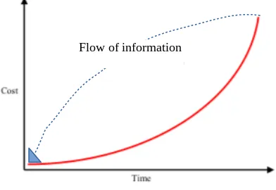
The presence of bugs in any written software in inevitable. However, the cost of fixing these bugs varies significantly, depending on when the bug is detected. Boehm’s cost of change curve (Figure 1) is an exponential curve, implying that the cost of fixing a bug at a given stage will always be greater than the cost of fixing it at an earlier stage (Boehm, 1976). Hence, if software developers are able to detect bugs at an earlier stage, the cost incurred in fixing the bug would be significantly lower.
More recent trends revolve around the fact that bugs can now be predicted, much before they are detected. So, by determining the presence or absence of a bug in a software release, developers can predict the success of a software release even before it is released, based on a few features (characteristics) of the release version. If this prediction is performed at a stage earlier than production in the software development cycle, it will reduce the cost of fixing
the bug. Moreover, if the information available at the production stage of a version release is fed back (Ambler, 2009) to the requirements stage (Figure 2), we might be able to develop a bug prediction model efficient enough to be used commercially in the software development industry.
This prediction can be done using machine learning techniques. This paper uses Microsoft’s popular MLaaS cloud tool Azure to make these predictions and compare the results.
This paper goes on to propose the use of machine learning as a service (MLaaS) to provide a viable solution to software developers for predicting the presence of bugs in the written software, thereby providing Bug Prediction as a Service (BPaaS).
2
LITERATURE REVIEW
Software companies around the world use predictive analysis to determine how many bugs will appear in the code or which part of the code is more prone to bugs. This has helped cut down losses due to commercial failure of software releases. However, the extent to which these measures reduce the cost of changing the code is yet to be explored. By looking at the cost of change curve (Boehm, 1976; Beck, 1999) for various software development methods it is evident that the earlier a bug is fixed, the less it will cost a company to rectify the bug. More recently, service oriented computing allows for software to be composed of reusable services, from various providers. Bug prediction methods can thus be provided as a reusable service with the help of machine learning on the cloud.
2.1 Early use of machine learning
The use of machine learning to create an entirely automated method of deciding the action to be taken by a company when a bug is reported was first proposed by Čubranić and Murphy (2004). The method adopted uses text categorization to predict bug severity. This method works correctly on 30% of the bugs reported to developers. Sharma, Sharma and Gujral (2015) use feature selection to improve the accuracy of the bug prediction model. Info gain and Chi square selection methods are used to extract the best features to train a naive Bayes multinomial algorithm and a K-nearest neighbours algorithm.
2.2 Bug prediction
[image:3.595.72.271.247.382.2]The above mentioned methods work when the bug is directly reported, though they introduce the concept
Figure 1: The traditional cost of change curve
Figure 2: The traditional cost of change curve with feedback
[image:3.595.76.272.433.568.2]of machine learning for software defect classification. The following papers aim to predict the presence of a bug in the software release.
Sivaji et al. (2015) envisions bug prediction methods being built into the development environment for maximum efficiency. This requires an exceptionally accurate model. They weigh the gain ratio of each feature and select the best features from the dataset to predict bugs in file level changes. They conclude that of the entire dataset, 4.1 – 12.52 % of the total feature set yields the best result for file level bug prediction. Zimmermann, Premraj and Zeller (2007) address the important question – which component of a buggy software actually contains the defect. It analyses bug reports at the file and package level using logistic regression models. The use of linear regression to compute a bug proneness index is explored by Puranik, Deshpande and Chandrasekharan (2016). They perform both linear and multiple regression to find a globally well fitting curve for the dataset. This approach of using regression for bug prediction did not yield convincing results. In agreement with Challagulla et al. (2005), since one prediction model cannot be prescribed to all datasets, this paper documents the evaluation metrics of various prediction models. This paper too, did not find any significant advantage of using feature extraction and/or principle component analysis (PCA) on the dataset prescribed by D'Ambros, Lanza and Robbes (2010).
2.3 Dataset
An extensive study of the various methods of predicting bugs in class level changes of six open source systems was conducted by (D'Ambros, Lanza and Robbes, 2010). The paper proposed a dataset that would best fit a prediction model for bug prediction in class level changes of the Eclipse IDE. This dataset has been used for bug prediction in this paper. According to previous findings (Nagappan and Ball, 2005; Nagappan, Ball and Zeller, 2006) the dataset that was used to train the prediction model includes code churn as a major feature and is given due weightage. By including bug history data along with software metrics, in particular CK metrics in the dataset used for prediction, we hope to improve the prediction accuracy. In future we shall work towards overcoming the `lack of formal theory of program` in bug prediction as specified by Fenton and Neil (1999).
3
BUG PREDICTION IN
SOFTWARE DEVELOPMENT
3.1 Importance of Bug Prediction
A software defect may be an error in the code causing abnormal functionality of the software or a feature that does not conform to the requirements. Either way, the presence of a bug is undesirable in the commercial release of a software or a version thereof. The most common bugs occur during the coding and designing stages. The Software Fail Watch report- 5th edition (https://www.tricentis.com/
software-fail-watch, 2018) by a software company called Tricentis claimed that 606 reported software bugs had caused a loss of $1.7 trillion worldwide, in 2017. It is evident that an efficient means of predicting software defects will help cut down the loss due to software production globally.
3.2 Current Bug Prediction in the
Market.
The waterfall model of software development suggests testing for defects after integrating all of the components in the system. However, testing each unit or component after it has been developed increases the probability of finding a defect.
The iterative model incorporates a testing phase for each smaller iteration of the complete software system. This leads to a greater chance of finding the bugs earlier in the development cycle.
The V-model has intense testing and validation phases. Functional defects are hard to modify in this model, since it is hard to go back once a component is in the testing phase. The agile model also uses smaller iterations and a testing phase in each iteration.
The various prototyping models too have testing methods for each prototype that is created. From this, we can see that the testing phase is always done later on in the development cycle. This will inevitably lead to larger costs of fixing the defect.
traditional methods of software testing like black box, white box, grey box, agile and ad hoc testing.
3.3 Cost of Change
This paper works on two models trained on two different datasets of bug reports form an Eclipse version release. One model predicts the presence of a bug based only on the types of bugs found in versions before this release. This model can be used to fix a bug at the earliest stage, with minimal cost. The second model uses a dataset of CK metrics and code attributes to predict a defect. Though the second model has a slightly better performance, the details in the dataset used to train the second model will only be available to the developer during design or (worst case) after the coding stage.
This paper proposes two models – one based solely on previous version data and a second based on attributes of the class in the current version. If Ambler’s cost of change curve (Figure 3) is followed (for the agile software development cycle), the first model is preferred, since it can predict buggy code at an earlier stage. However, if Kent Beck’s cost of change curve (Figure 4) (Beck, 1999) for eXtreme Programming (XP) is followed, the second model’s higher AUC score (though available only at a later stage) might be more desirable, since the cost does not grow exponentially.
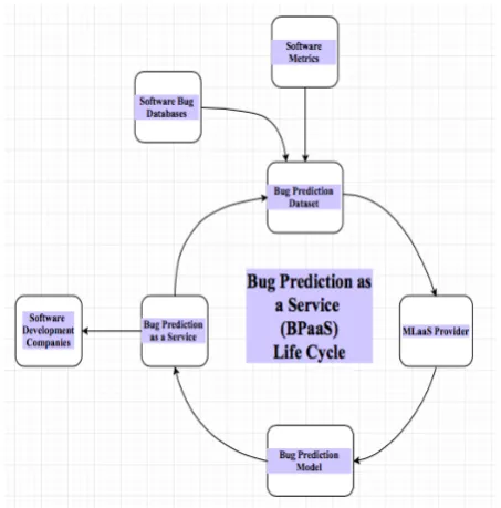
3.4 Bug Prediction as a Service
Figure 5 shows the schematic flowchart of the process of bug prediction using machine learning. The bug reports from various development environments along with various software metrics are stored in a bug database. This database is used to train a suitable machine learning model. By deploying the machine learning model on the cloud, bug prediction can be provided as a cloud based service to software development companies across the world.
4
DATASET
The models that this paper proposes are based on two different datasets, both of which are freely available at http://bug.inf.usi.ch. For this paper, the “Change metrics (15) plus categorized (with severity and priority) post-release defects” dataset for model 1 and the “Churn of CK and other 11 object oriented metrics over 91 versions of the system” dataset for model 2 have been used, but this method can easily be extended to any dataset required.
4.1 Model 1
[image:5.595.308.535.232.462.2]T
he “Change metrics (15) plus categorized (with severity and priority) post-release defects” dataset used to train the first model is described below:Figure 3: Ambler’s traditional cost of change curve
Figure 4: Kent Beck’s cost of change curve
[image:5.595.75.272.432.707.2]4.1.1 Description
The features in the dataset are: 1. classname
2. numberOfVersionsUntil 3. numberOfFixesUntil
4. numberOfRefactoringsUntil 5. numberOfAuthorsUntil 6. linesAddedUntil 7. maxLinesAddedUntil 8. avgLinesAddedUntil 9. linesRemovedUntil 10. maxLinesRemovedUntil 11. avgLinesRemovedUntil 12. codeChurnUntil 13. maxCodeChurnUntil 14. avgCodeChurnUntil 15. ageWithRespectTo
16. weightedAgeWithRespectTo 17. bugs
18. nonTrivialBugs 19. majorBugs 20. criticalBugs 21. highPriorityBugs
Since this paper aims to detect the presence or absence of bugs in a software release, we replace columns 17, 18, 19, 20 and 21 with a single column. Let the name of the column be ‘clean’; it will take the value 1 if there are no bugs in the code, and a value 0 if at least one bug exists in the software.
4.2 Model 2
The “Churn of CK and other 11 object oriented metrics over 91 versions of the system” dataset used to train model 2 uses CK metrics to predict the presence of bugs in a software release.
4.2.1 CK metrics
Code churn refers to the amount of change made to the code of a software system / component. This is used along with CK metrics in this dataset. The Chidamber and Kemerer metrics were first proposed in 1994, specifically for object oriented design of code. The CK metrics are explained in Table 1.
CBO (Coupling between Objects) CBO is
the number of classes that a given class is coupled with. If a class uses variables of another class or calls methods of the other class, the classes are said
to be coupled. The lower the CBO, the better, since the independence of classes decreases with increase in coupling.
DIT (Depth of Inheritance Tree) DIT is the
number of classes that a given class inherits from. DIT should be maximal because a class is more reusable, if it inherits from many other classes.
LCOM (Lack of Cohesion of Methods)
LCOM is the number of pairs of functions that access the same data (i.e.,) variables. A larger LCOM indicates more cohesion, which is more desirable.
NOC (Number of Children) NOC is the
number of immediate subclasses to a class. NOC is directly proportional to the reusability, since inheritance is a form of reuse (Bieman and Zhao, 1995). Hence, NOC should be large.
RFC (Response For Class) RFC is the sum
of the number of methods in the class and the number of methods called by the class. A large RFC is usually the result of complex code, which is not desirable.
WMC (Weighted Methods for Class) WMC
is a measure of the total complexity of all the functions in a class. WMC must be low for the code to be simple and straightforward to test and debug.
4.2.2 Description
The features in the dataset are:
1. classname 2. cbo 3. dit 4. fanIn 5. fanOut 6. lcom 7. noc
8. numberOfAttributes
9. numberOfAttributesInherited 10. numberOfLinesOfCode 11. numberOfMethods
12. numberOfMethodsInherited 13. numberOfPrivateAttributes 14. numberOfPrivateMethods 15. numberOfPublicAttributes 16. numberOfPublicMethods 17. rfc
18. wmc 19. bugs
20. nonTrivialBugs 21. majorBugs 22. criticalBugs 23. highPriorityBugs
Column 4 fanIn refers to the count of classes that access a particular class, while Column 5 fanOut is
for every entry i in the dataset: clean
the number of classes that are accessed by the class under study. Here, accessing a class could mean calling a method or referencing a variable.
Again, to detect the presence or absence of bugs in a software release, we replace columns 19, 20 and 21, 22, 23 with a single column. Let the name of the column be ‘clean’; it will take the value 1 if there are no bugs in the code, and a value 0 if at least one bug exists in the software.
5. EXPERIMENT
5.1 MLaaS
Machine Learning as a Service is a term used for the cloud services that provide automated machine learning models with in-built preprocessing, training, evaluation and prediction modules. Some of the forerunners in this domain are Amazon’s Machine Learning services, Microsoft’s Azure Machine Learning and Google’s Cloud AI, to name a few. MLaaS has a huge potential (Yao et al., 2010) and is also much easier to deploy as a web service, for software companies worldwide.
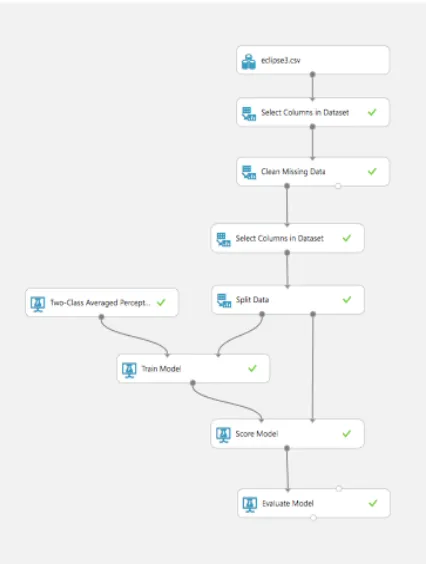
5.2 Microsoft Azure
Azure is Microsoft’s cloud computing service which provides a wide variety of services globally. The Azure ML Studio is a component of the Cortana Intelligence Suite for predictive analysis and machine learning. It has a user friendly interface and allows for easy testing of a number of machine learning models provided by the studio. Azure provides an option to set up a web service, in turn allowing bug prediction to be provided as a service on the cloud. A schematic flowchart for the process is shown in Figure 6.
5.3 Machine Learning Models
The four categories of machine learning models offered by Microsoft Azure are Anomaly detection, Classification, Clustering and Regression. Anomaly detection is usually used to detect rare, unusual data entries from a dataset. Classification is used to categorize data. Clustering groups the data into as many sets as it may hold, usually useful for discovering the structure of the dataset. Regression is used to predict a value in a specified range.
Therefore, we use binomial classification for both the models to categorize our dataset into two classes – buggy or clean.
6. RESULTS
6.1 Metrics
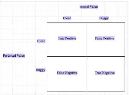
Each predicted outcome of the experiment (i.e.,) the code is clean or buggy can be classified under one of the following types:
1. True Positive (TP) 2. True Negatives (TN) 3. False Positives (FP) 4. False Negatives (FN)
The definition of each type is given in Figure 7.
The criteria used to evaluate the classification model are:
Accuracy:
Accuracy is the ratio of correct predictions to the total number of predictions.
Accuracy =
for every entry i in the dataset: clean
i = 1 , if bugsi =0 0, otherwise
Figure 6: Schematic flowchart of the machine learning experiment in Azure.
[image:7.595.310.523.91.373.2] Precision
Precision is the proportion of the positive predictions that are actually positive.
Precision =
Recall
Recall is the proportion of the positive observations that are predicted to be positive.
Recall =
F1 Score
F1 score is the harmonic average of the precision and the recall. It is not as intuitive as the other metrics, however it is often a good measure of the efficiency of the model. F1 score is a good metric to
follow if both false positives and false negatives have the same cost (or here, loss incurred by the company).
F1 Score =
Area Under the Receiver Operating Curve
The AUC denotes the probability that a positive prediction chosen at random is ranked higher than a negative prediction chosen at random by the model.
6.2 Obtained Results
There are nine models offered by Azure ML Studio for binomial classification. They are logistic regression, decision forest, decision jungle, boosted decision tree, neural network, averaged perceptron, support vector machine, locally deep support vector machine and Bayes’ point machine.
The results from training model 1 and model 2 on each of the nine models are tabulated in Table 1 and Table 2 respectively.
The threshold is a measure of trade off between false positives and false negatives. Here, a false positive would be a clean software version being classified as buggy. This is of great burden on the developer who ay spend hours searching for a bug that does not exist. A false negative would mean a bug in the release, which is a bother to the end user. Assuming the loss due to both these situations is the same, the threshold was set to 0.5.
6.3 Interpretation
From Table 1 and table 2, we conclude that a two class averaged perceptron model for the first dataset
Figure 7: Classification of Predicted Outcomes.
(TP
)
(
TP+FP
)
(TP
)
(TP+FN
)
[image:8.595.74.284.92.247.2](
2
∗Recall∗Precision
)
(
Recall+Precision)
and a two class decision jungle for the second dataset are the best suited.
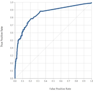
The ROC curves for both the datasets are plotted in Figure 8 and Figure 10. The high area under the ROC curve indicates a high chance that a
positive prediction chosen at random will be ranked higher than a negative prediction chosen at random.
[image:9.595.325.523.330.688.2] [image:9.595.327.521.331.491.2]The Precision-Recall curves are plotted in Figure 9 and Figure 11. The area under the precision recall graph in very high in Figure 9 denoting a high
Table 2 : Results obtained from various classification models with training dataset 2.
Figure 8 : The ROC curve for model 1
[image:9.595.105.269.337.495.2]Figure 10 : The ROC curve for model 2
Figure 9 : The Precision-Recall curve for model 1
[image:9.595.331.521.504.689.2] [image:9.595.98.259.529.688.2]precision and a high recall. Since high precision corresponds to a low FP rate and high recall corresponds to a low FN rate, this denotes that this model is very accurate. These graphs are plotted by the Microsoft Azure ML Studio under the option ‘Evaluate model’.
We have given equal weightage to all five evaluation metrics used in this paper, and have decided upon a suitable model. However, the metrics for various models have all been documented for comparison. A software tester may feel that a different evaluation metric describes his needs better, for instance when a false positive costs more than a false negative or vice versa. In such cases, the machine learning model can easily be switched for a more suitable machine learning model. This is the advantage of using machine learning as a service (MLaaS) on the cloud for bug prediction.
7. CONCLUSION AND FUTURE
WORK
The model proposed by this paper has an F1 score of 91.5% for model 1, which works with only previously known data, so as to predict the presence of a bug in the earliest possible stage of software development. This is more suitable for agile software development, where the F1 score combined with a reduced cost of rectifying the defect (according to Ambler’s cost of change curve) is profitable. The second model proposed uses a two class decision jungle model with an F1 score of 90.7%. This model uses details known at design and coding phase, to predict the presence of a bug and can be used in XP development due to the level increase in the cost of change curve. The accuracy and precision of the models in this paper are high enough for these models to be commercially used in software development companies. Moreover, the memory footprint of the two class decision jungle is lower than any other model. Future work may include increasing the accuracy of these models with commercial datasets (as opposed to the open-sourced datasets used in this experiment). The use of MLaaS in this paper allows the bug prediction models to be deployed on the cloud, as a service. When these models are provided as a web service on the cloud, the proposed model of Bug Prediction as a Service becomes a viable option for software development companies.
8. REFERENCES
Boehm, B., 1976. ‘Software Engineering and Knowledge Engineering’, Proceedings of IEEE Transactions on Computers. IEEE, pp. 1226–1241.
Scott W. Ambler. 2009. Why Agile Software
Development Techniques work: Improved feedback. [ONLINE] Available at: http://www.ambysoft.com. Čubranić, D. & Murphy, G. C., 2004. ‘Automatic bug
triage using text classification’, Proceedings of Software Engineering and Knowledge Engineering. pp. 92–97.
Sharma, G., Sharma, S. & Gujral, S., 2015. ‘A Novel Way of Assessing Software Bug Severity Using Dictionary of Critical Terms’, Procedia Computer Science, 70, pp.632–639.
Shivaji, S. et al., 2009. Reducing Features to Improve Bug Prediction, Proceedings of IEEE/ACM International Conference on Automated Software Engineering. pp. 600–604.
D'Ambros, M., Lanza, M. & Robbes, R., 2010. An extensive comparison of bug prediction approaches.
Proceedings of the 7th IEEE Working Conference on Mining Software Repositories (MSR).
Puranik, S., Deshpande, P. & Chandrasekaran, K., 2016. A Novel Machine Learning Approach for Bug Prediction.
Procedia Computer Science, pp.924–930. Zimmermann, T., Premraj, R. & Zeller, A., 2007.
Predicting Defects for Eclipse. Proceedings of the Third International Workshop on Predictor Models in Software Engineering. p. 9.
Fenton, N.E. & Neil, M., 1999. ‘A critique of software defect prediction models’, Proceedings of IEEE Transactions on Software Engineering, pp. 675–689. Challagulla, V. U. B., Bastani, F. B.; Yen, I-Ling, Paul, R.
A., (2005). ‘Empirical assessment of machine learning based software defect prediction techniques’,
Proceedings of the 10th IEEE International Workshop on Object-Oriented Real-Time Dependable Systems. pp. 263-270.
Nagappan, N. & Ball, T., 2005. ‘Use of Relative Code Churn Measures to Predict System Defect Density’,
Proceedings of the 27th international conference on Software engineering, St. Louis, pp. 284–292. Nagappan, N., Ball, T. & Zeller, A., 2006. ‘In Mining
metrics to predict component failures’, Proceedings of the 28th international conference on Software engineering, Shanghai, pp. 452–461.
Tricentis, 2018. Software Fail Watch: 5th Edition, Tricentis. Available at:
https://www.tricentis.com/software-fail-watch. Yao, Y et al., 2010. Complexity vs. performance:
empirical analysis of machine learning as a service.
Proceedings of the Internet Measurement Conference. pp. 384–397.
IEEE Transactions on Software Engineering, 20(6), pp. 476-493.
Hand, D.J. & Till, R.J., 2001. A Simple Generalisation of the Area Under the ROC Curve for Multiple Class Classification Problems. Machine Learning, 45(2), pp.171–186.
Hassan, A.E. & Holt, R.C., 2005. ‘The top ten list: dynamic fault prediction’, Proceedings of the 21st IEEE International Conference on Software Maintenance, pp. 263–272.
Beck, K., 1999. Extreme programming explained: embrace change, Boston, MA: Addison-Wesley Longman.