A Review on Attempts towards CAD/CAE Integration Using Macroelements

A Review on Attempts towards CAD/CAE Integration

Using Macroelements

Christopher Provatidis

National Technical University of Athens, Greece *Corresponding Author: [email protected]

Copyright © 2013 Horizon Research Publishing All rights reserved.

Abstract

In this paper we review several aspects of older and contemporary attempts to integrate computer-aided design (CAD: geometric model) and computer-aided engineering (CAE: finite elements, boundary elements, etc.). After a short review on formulas for the description of CAD surfaces, a systematic mechanism for creating several types of corresponding isoparametric macroelements is presented. Gordon-Coons is initially applied in conjunction with piecewise linear, Lagrange polynomials and natural B-splines. Then, it is extended to more basis and blending functions. In addition to the well-known ‘Lagrangian’-type elements, equivalent ‘Bézierian’-type elements are introduced. Tensor product B-splines and aspects of NURBS isogeometric formulation are given. In addition to quadrilaterals, triangular macroelements based on Barnhill’s interpolation are presented for the first time. The review covers applications of CAD-based macroelements in conjunction with the Galerkin-Ritz formulation, the Boundary Element Method, as well as recent Global Collocation procedures. A numerical example on a vibrating membrane elucidates the performance of the CAD-based global interpolation and depicts its superiority over the conventional finite element method.

Keywords

CAD, CAE, Global Interpolation, Finite Element, Boundary Element, Collocation Techniques

1. Introduction

Computer-Aided Design (CAD) is the use of computer systems to assist in the creation, modification, analysis, or optimization of a design. One the earliest personalities who have contributed in this area, and had a vision of interactive computer graphics as a powerful design tool, were Steven Anson Coons (1912 – 1979), a professor in the Mechanical Engineering Department at Massachusetts Institute of Technology (MIT) during the 1950s and 1960s. During World War II, he worked on the design of aircraft surfaces,

developing the mathematics to describe generalized “surface patches”. At MIT’s Electronic Systems Laboratory he investigated the mathematical formulation for these patches, and in 1967 published one of the most significant contributions to the area of geometric design, a treatise which has become known as “The Little Red Book” [1]. His “Coons Patch” was a formulation that presented the notation, mathematical foundation, and intuitive interpretation of an idea that would ultimately become the foundation for other surface descriptions that are commonly used today, such as B-spline surfaces, NURB surfaces, etc. His technique for describing a surface was to construct it out of collections of adjacent patches, which had continuity constraints that would allow surfaces to have curvature which was expected by the designer. Each patch was defined by four boundary curves, and a set of “blending functions” that defined how the interior was constructed out of interpolated values of the boundaries. The interested reader may find more details in [2].

Computer-Aided Engineering (CAE) is the broad usage of computer software to aid in engineering tasks. It includes computer-aided design (CAD), computer-aided analysis (CAA), computer-integrated manufacturing (CIM), computer-aided manufacturing (CAM), material requirements planning (MRP), and computer-aided planning (CAP). In a more strict sense, CAE areas include:

 Stress analysis on components and assemblies using FEA (Finite Element Analysis);

 Thermal and fluid flow analysis Computational fluid dynamics (CFD);

 Multibody dynamics (MBD) & Kinematics;  Analysis tools for process (manufacturing)

simulation for operations such as casting, molding, and die press forming.

 Optimization of the product or process.

 Safety analysis of postulate loss-of-coolant accident in nuclear reactor using realistic thermal-hydraulics code.

 Pre-processing – defining the model and

environmental factors to be applied to it (typically a finite element model, but facet, voxel and thin sheet methods are also used).

 Analysis solver (usually performed on high powered computers).

 Post-processing of results (using visualization tools). This cycle is iterated, often many times, either manually or using built-in procedures, or finally by linking the entire procedure into a commercial optimization software such as [3, 4].

Henceforth, CAE will restrict to the finite element (FEM/FEA) and the boundary element (BEM) analysis, whereas a very recent Global Collocation Method (GCM) will be reviewed and commented. It is reminded that FEM decomposes the model of the structure in small areas or volumes, called finite elements [5, 6], whereas BEM deals mostly with the boundary of the structure [7].

It is accepted that the pioneers in the FEA area are John HadjiArgyris (1913–2004), Olgierd Cecil Zienkiewicz (1921–2009) and Ray Clough (1920–today). Some personal views are [8-12].

The decade of 1960s was very important for designers, as since then they have long used computers for their calculations. Initial developments were carried out in the 1960s within the aircraft and automotive industries in the area of 3D surface construction and NC programming, most of it independent of one another and often not publicly published until much later. Some of the mathematical description work on curves was developed in the early 1940s by Isaac Jacob Schoenberg, Apalatequi (Douglas Aircraft) and Roy Liming (North American Aircraft), however probably the most important work on polynomial curves and sculptured surface was done by Pierre Bézier (Renault), Paul de Casteljau (Citroen), Steven Anson Coons (MIT, Ford), James Ferguson (Boeing), Carl de Boor (GM), Birkhoff (GM) and Garabedian (GM) in the 1960s and W. Gordon (GM).

It is argued that a turning point was the development of SKETCHPAD system in MIT in 1963 by Ivan Sutherland [13], who was a student of S.A. Coons; however his PhD thesis was supervised by C.E. Shannon (1916 –2001), the "father of information theory". The distinctive feature of SKETCHPAD was that it allowed the designer to interact with his computer graphically: the design can be fed into the computer by drawing on a CRT monitor with a light pen. Effectively, it was a prototype of graphical user interface (GUI), an indispensable feature of modern CAD.

First commercial applications of CAD were in large companies in the automotive and aerospace industries, as well as in electronics. Only large corporations could afford the computers capable of performing the calculations. Notable company projects were at GM (Dr. Patrick J.Hanratty) with DAC-1 (Design Augmented by Computer) 1964; Lockhead projects; Bell GRAPHIC 1 and at Renault (Bézier) UNISURF 1971 car body design and tooling. One of the most influential events in the development of CAD was the founding of MCS (Manufacturing and Consulting

Services Inc.) in 1971 by Dr. P. J. Hanratty[14], who wrote the system ADAM (Automated Drafting And Machining) but more importantly supplied code to companies such as McDonnell Douglas (Unigraphics), Computer vision (CADDS), Calma, Gerber, Autotrol and Control Data. As computers became more affordable, the application areas have gradually expanded. The development of CAD software for personal desk-top computers was the impetus for almost universal application in all areas of construction. Other key points in the 1960s and 1970s would be the foundation of CAD systems United Computing, Intergraph, IBM, Intergraph IGDS in 1974 (which led to Bentley MicroStation in 1984) CAD implementations have evolved dramatically since then. Initially, with 2D in the 1970s, it was typically limited to producing drawings similar to hand-drafted drawings. Advances in programming and computer hardware, notably solid modeling in the 1980s, have allowed more versatile applications of computers in design activities.

Key products for 1981 were the solid modelling packages -Romulus (ShapeData) and Uni-Solid (Unigraphics) based on PADL-2 and the release of the surface modeler CATIA (Dassault Systemes). Autodesk was founded 1982 by John Walker, which led to the 2D system AutoCAD. The next milestone was the release of Pro/ENGINEER in 1988, which heralded greater usage of feature-based modeling methods and parametric linking of the parameters of features. Also of importance to the development of CAD was the development of the B-rep solid modeling kernels (engines for manipulating geometrically and topologically consistent 3D objects) Parasolid (ShapeData) and ACIS (Spatial Technology Inc.) at the end of the 1980s and beginning of the 1990s, both inspired by the work of Ian Braid. This led to the release of mid-range packages such as SolidWorks in 1995, SolidEdge (Intergraph) in 1996, and IronCAD in 1998. Nowadays CAD is one of the main tools used in designing products.

In order to analyze mechanical components, which are usually characterized by complex shapes, the computer-aided-design (CAD) model is usually exported in the form of a neutral file (IGES, DXF, STEP) that is further imported by a selective finite element (FEM) or boundary element (BEM) code. This procedure induces some difficulties such as the appearance of double points (or double lines) or loss of at least a few geometrical data. Of course, specific CAD converters such as PATRAN can export many types of FEM data that can be immediately feed commercial FEM codes. Specialized CAD/CAM/CAE integrated systems such as PRO/ENGINEER, IDEAS and Dassault Systèmes (SOLIDWORKS, PLM: Product Lifecycle Solutions) exist for the last 20 or 25years. However, in all these tools the computational mesh generation is a time-consuming task that has to follow the creation of the CAD model. A survey of thirty-four finite element systems until 1981 was reported by Brebbia [15].

tube size for the skeleton of the structure (CAD); then, an integrated CAD/CAE system has to automatically understand not only the diameter and the thickness but also the second moment of inertia of this tube, without the engineer having to perform the relevant numerical calculations. Closely related, the engineer can generate the mesh without exiting the CAD system and then entering the CAE system; in other words, both systems are integrated in one, sharing the same database as is possible.

A second point of view is the usually reported fact that the CAD/CAE integration and scientific visualization is related to both the reduction of errors in the information transfer from system to system as well as the reduction of memory resources and overall computational time [16, 17]. The ‘vehicle’ for CAD/CAE integration is to use a common platform to describe the geometry and the unknown variable that satisfies a partial differential equation (PDE) of a multi-physics boundary-value-problem (e.g. heat transfer, elastostatics, thermo-elasticity, fluid mechanics, electromagnetic, etc). A third point of CAD/CAE integration is to replace the usual finite elements (of small-size) with others of larger size applying the same interpolation for both the geometry and the variable. Relevant macro-elements are usually of “isoparametric” type whereas “isogeometric” ones have appeared [18].

The lack of a complete, synthetic and critical report on the abovementioned third point of CAD/CAE integration, which is directly related to the development and use of macroelements, has motivated the author to write this review article.

The paper is structured as follows. Section 2 summarizes the one-dimensional (univariate) interpolation as well as the five basic CAD formulations. Section 3 reviews the usual applications in which Coons’ interpolation has been used, as well as the derivation of global shape functions. Section 4 provides details about the isoparametric or isogeometric-like approximation that is used for the interpolation of both the geometry and the variable or the unknown coefficients. Section 5 reviews the three possible computational methods to be applied in conjunction with the global interpolation within subregions, and provides the numerical procedure for the estimation of mass and stiffness matrices of the structure. Section 6 presents original numerical results concerning the extraction of natural frequencies for a fixed rectangular membrane. Section 7and Section 8are the “Discussion” and the “Conclusions”, respectively.

2. CAD Surface Interpolations

2.1. General

Historically, there are rather five main interpolation formulations in CAD theory [19]: (i) Coons interpolation, (ii) Gordon-Coons interpolation, (iii) Bézier interpolation, (iv) B-splines interpolation, and (v) NURBS. The first two of

them directly refer to the coordinates of nodal points that belong to the boundary or the interior of a patch, whereas the last three refer to control points (at the edges of polygonal generators that generally do not belong to the curvilinear boundary). In all five cases the interpolation of geometry refers to the coordinates of either nodal points or control points multiplied by proper basis functions. For the sake of completeness, we start with one-dimensional and then extend to two- and three-dimensional interpolation.

2.2. One-Dimensional Interpolation

Let us consider the domain a≤x≤b in which we wish to interpolate the function f(x).

Among others, the most usual interpolations of the function f(x) are: (i) Power series, (ii) Lagrange polynomials, (iii) Legendre polynomials (p-method), (iv) Chebyshev polynomials, (v) Bernstein polynomials (Bézier curve), (vi) B-splines, and (vii) NURBS. All of them will be briefly described below.

2.2.1. Power Series

The function is approximated by:

( )

0 1

0

n

n j

n j

j

f x

a a x

a x

a x

=

=

+

+ +



≡

∑

(1)

2.2.2. Lagrange Polynomials The function is approximated by:

( )

( )

( )

( )

0 0

n n

j j j j

j j

f x

L x f x

L x f

= =

=

∑

≡

∑

(2)

where

L x

_j

( )

denotes the well-known Lagrange polynomial (see, for example, [20]).

2.2.3. P-Method

The relevant series expansion includes the nodal values at the ends, f(a) and f(b) for which the classical linear hat functions are considered, i.e.: N x1

( )

= −1 x L and

( )

2 1

N x = −x L where

L b a

= −

. In addition, we define a certain polynomial degree ‘p’, which leads to a number of functions

φ

_j are defined in terms of the Legendre polynomial

P

_j−₁:

( )

₁ 1

( )

2 1

,

2,3,

2

x

j j

j

x

P t dt j

φ

₋

−

−

=

∫

=

_

(3)

It is reminded that the Legendre polynomials are given by

( )

1

(

2

₁

)

2

!

m

m

m m m

d

P x

x

m dx

=

−

,(4)

and they are solutions of the ordinary differential operation:

It is also reminded that the well-known Gauss points are roots of the above Legendre polynomials.

The basis functions N1, N2 are called nodal shape

functions or external shape functions or external modes. The basis functions Ni =

φ

i−1,i=3, 4, , p+1 are called internal shape functions or internal modes, or, sometimes, “bubble modes”.

Therefore:

( )

1

( )

1 2

( )

2 1

( )

3

p

j j j

f x

N x f N x f

+

N x a

=

=

+

+

∑

(6)

The advantage of these functions is that they are orthogonal thus leading to banded mass and stiffness matrices [21, pp. 37-47].

2.2.4.ChebyshevPolynomials

Although these polynomials do not directly appear in CAD formulations, it is instructive to mention that they can approximate a function with the same accuracy with the power series. They are categorized in polynomials of first and second kind. For example, the Chebyshev polynomials of the second kind are defined as:

( )

{

(

₍

)

₎

}

(

)

(

)

1

1

2 2

2

4 2

sin

1 cos

sin cos

1

1

1

1

3

1

1

5

m

m m

m

m

x

U x

x

m

m

x

x

x

m

x

x

− −

−

−

+

=

+

+

=

−

−

+

+

−

−







































(7)

and their roots are given by

(

)

ˆ cos

,

1, , .

1

i

i

_i

_m

m

π

ξ

=

=

+



(8)

As we will see later, the above roots can be used as collocation points in a global collocation method, which is an alternative to the Galerkin-Ritz procedure [22, 23].

2.2.5. Bernstein Polynomials (Bézier curve) 2.2.5.1. Nonrational Bézier Curve

A curve of n-th degree is defined as

( )

,

( )

0

0 1

n

i n i

i

u B u u

=

=

∑

≤ ≤

C P (9)

where C

( )

u =

[

x u

( )

y u

( )

]

T are the Cartesian coordinates on the xy-plane.

The basis functions, Bi n,

( )

u , are the classical Bernstein

polynomials that are defined as

( )

(

)

(

)

(

)

,

!

1 1

! !

n i n i

i i

i n

n n

B u u u u u

i i n i

− −

= − = −

−

 

 

 

(10)

The geometrical coefficients,

{ }

Pi , are called control points. Equation (10) denotes that for a curve that is determined by (n + 1) control points, the term of highest degree is

u

n. This implies that the polynomial degree of Bézier curve is determined by the number of control points. The basic properties of a Bézier curve are many and can be found elsewhere [24-27]. In brief:

 The curve passes through the first (Ρ0) and the last

(Ρn) control points and its tangent at these ends has

the direction of the first straight segment (Ρ0Ρ1) and

the last one (Ρn-1Ρn), respectively, of the control

polygon (Ρ0Ρ1… Ρn-1Ρn).

 The Bernstein polynomials are nonnegative:

( )

,

0

i n

B u

≥

 They have the rigid-body property (partition of unity:

( )

[ ]

, 0

1, 0,1

n

i n i

B u u

=

= ∀ ∈

∑

).

 They are smaller than unit except of those associated to the ends where they equal to unity, and appear a maximum in the interval [0,1] at utan 0= =i n.

 They are symmetric with respect to the position

1 2,

u

=

∀

n

.

 They are rapidly calculated by the following recursive formula:

( ) (

)

( )

( )

( )

, , 1 1, 1

,

1

,

0(

0,

)

i n i n i n

i n

B u

u B

u

uB

u

B u

i

i n

− − −

= −

+

≡

<

>

.(11)

 Their derivative is also calculated by the following recursive formula:

( )

( )

(

( )

( )

)

( )

( )

,

, 1, 1 , 1

1, 1 , 1

.

,

0

i n

i n i n i n

n n n

dB u

B u

n B

u

B

u

du

B

u

B

u

− − − − − −

′

=

=

−

≡

≡

(12)

It is also remarkable that:

 The time-consuming computation of the i-combinations

n

i

 

 

 

is simplified by using

Casteljau’s algorithm.

 Also, the interpolation of Bézier curve is mathematically equivalent with the power series (1), for the same value of n.

 Similarly, both the p-method and the Bernstein polynomials are equivalent with the Lagrange polynomials [see, (2)], of course for the same value of n.

2.2.5.2. Rational Bézier Curve

Since the conical surfaces, i.e. circles, ellipses, hyperbolas, cylinders, cones, spheres, et cetera, are not described precisely by means of polynomials, but require the use of rational functions, the form:

( )

X u

( )

_{( )}

,

( )

Y u

( )

_{( )}

x u

y u

W u

W u

it became necessary to introduce the n-th rational Bézier curve, which is defined as:

( )

{

( ) ( )

}

( )

{

}

( )

, 0 , 0 , ,

, 0 1

n

i n i i i i

i n

i n i

i C u x u y u

B u w P x y

u B u w

= = = ⋅ ⋅ = ≤ ≤ ⋅

∑

∑

(14) or

( )

,

( )

0

, 0 1

n

i n i

i

u R u u

=

=

∑

⋅ ≤ ≤

C P ( (15)

where

( )

( )

( )

, , , 0

, 0 1

i n i

i n n

j n j

j

B u w

R u u

B u w

=

⋅

= ≤ ≤

⋅

∑

(16)

2.2.6. B-Splines

2.2.6.1. Older Definitions

The meaning of splines was published in 1946 and later by Schoenberg [28]. It refers to the points

0 0 1 1

( , ),( , ), ,( , )x f x f … x fn n with x0 <x1<< xn ,

which we wish to interpolate through a multiply-defined function f x

( )

. The points x x0, , ,1  xn are called

“breakpoints”. For the sake of briefness and without loss of generality, we reduce to (cubic) polynomials of third degree. The desired properties are as follows:

 In each interval

x

_i−₁

≤ ≤

x x

_i, with i=1, 2, , n,

the function f x

( )

is a cubic polynomial.  The function f x

( )

, as well as the first and second

derivatives, are continuous at the above points. Introducing the truncated power as:

(

)

0,

,

i m i m i i

x x

x x

x x

x x

+

≤

−

=

−

>







, (17)

which has C(m-1)_{-continuity, the original expression consists}

of a power series in the form [28]:

( )

2 3 1 3

0 1 2 3

1

n

j j

j

f x a a x a x a x − b x x

= +

= + + + +

∑

− (18)

It is apparent that (18) includes (n+3) terms and ensures C2_{-continuity, because for simplicity we considered m = 3.}

Alternatively, (18) can be modified so as to include additional truncated polynomials of second degree, i.e.:

( )

2 3

0 1 2 3

2 3

1 1

1 1

n _{j j} n _{j j}

j j

f x

a a x a x

a x

b x x

c x x

− −

= + = +

=

+

+

+

+

∑

−

+

∑

−

, (19)

Obviously, (19) includes 2(n+1) terms and ensures C1_-continuity.

2.2.6.2. Contemporary Procedures

The breakthrough was made in 1972, independently by Cox [29] and DeBoor [30], who both achieved the B-splines and their derivatives to be rapidly computed through recursive formulas [including (11) and (12)]. Charles DeBoor [26] continued his research and his initial FORTRAN codes exist today in MATLAB (spline toolbox) under the name ‘spcol’, among others [31].

In brief, for a nondecreasing set of (n+1) breakpoints (

x x

₀

, , ,

₁



x

n−₁

,

x

n), and for a concrete polynomial degree

‘p’, we define the knot vector ‘U’, which strongly depends on the multiplicity of the internal nodes, as follows:

( ) ( )

( )



( )

0 0 1 1

1 terms 1 term

0 0 1 1 1 1

2 terms

1 terms 2 terms 1 term

, , , , , , , multiplicity 1

, , , , , , , , , , multiplicity 2

n n n

p p s

n n n n

p p s

x x x x x x U

x x x x x x x x

− + + − − + + = = =







_

_



_

_



_

_

_

_

























     







 

(20) Based on either of the knot vectors of (20), (m+1) control points (Ρ0 Ρ1… Ρm-1Ρm) are constructed, so as the following

relationship always holds:

1

m n p

= + +

₍₂₁₎

Let us consider a nondecreasing sequence

{

0, , m

}

U = u  u of real numbers, for example,

1, 0, , 1

i i

u ≤u+ i=  m− . The elements ui are called knots,

and U is the knot-vector. The i-th B-splines basis functions of degree p (order p+1), denoted by

N

_{i p,}

( )

u

, is defined as:

( )

( )

( )

( )

1 ,0

1

, , 1 1, 1

1 1

1 if

0 otherwise

i i i i p i

i p i p i p

i p i i p i

u u u

N u

u

u

u u

N

u

N

u

N

u

u

u

u

u

+ + + − + − + + + +

≤ <

=

−

−

=

+

−

−







(22) 2.2.6.3. Contemporary Versus Older Definitions

Some young readers may believe that (22) is different than (18) or (19). However, for example in case of p = 3 (cubic splines), it is trivial to prove that:

 When the multiplicity equals to one, the (n+3) basis functions of (22) are equivalent (not identical) to those basis functions given by (18).

 When the multiplicity equals to two, the 2(n+1) basis functions of (22) are equivalent (not identical) to those basis functions given by (19).

 Therefore, a lot of research conducted in 1960s using the older framework ((18) and (19)) may be repeated on the new framework of (22).

2.2.7.NonUniform Rational B-Spline (NURBS) Curve Similarly to the rational Bézier curve [see, (16)], non uniform rational B-splines (NURBS) is an extension of the B-splines in the following form:

( )

( )

( )

, 0

, 0

n

i p i i

i n

i p i

i

N u w u

N u w

= =

=

∑

∑

P C

(23)

where {wi} are the weights. Usually, a = 0, b = 1 and wi> 0

for all i. Taking the rational basis functions as,

( )

( )

( )

, ,

, 0

i p i

i p n

j p j

j

N u w R u

N u w

=

=

∑

, (24)

the curve is expressed as:

( )

,

( )

0

n

i p i i

i

u R u w

=

=

∑

C P

(25) and they are piecewise rational functions in the interval

[ ]

0,1 u∈ .

2.2.8. Comparison between Different Sets Of Basis Functions

It is well known that power series is identical with Lagrange polynomials [24, pp. 304-308]; the only difference is that the first includes arbitrary coefficients, whereas the second cardinal shape functions (of [1,0]-type) that are multiplied by the associated nodal values.

Chebyshev polynomials are also multiplied by arbitrary coefficients and they may have some advantages when collocating at their roots [22, 23].

The use of Legendre polynomials is somehow different. The relevant series expansion includes the nodal values at the ends, f(a) and f(b) for which the classical linear hat functions are considered, i.e.: N x1

( )

= −1 x L and

( )

2 1

N x = −x L where

L b a

= −

. In addition, a certain desired number of “bubble” functions, in the form of differences between Legendre polynomials, are usually used. The advantage of these functions is that they are orthogonal thus leading to banded matrices [21, pp. 39-46].

Bernstein polynomials have been used in the construction of the well-knownBézier curves, and can be found in many textbooks such as [25-27].

B-splines is nothing new but the usual spline interpolation, which can be found in every textbook of numerical analysis such as [20], whereas detailed information is given elsewhere [27-30]. The superiority of B-splines is that it can handle every high number of data, in contrast to Lagrange polynomials that cannot handle more than ten to twelve

points at maximum.

Finally, NURBS is an extension of B-splines as it uses weights for every control point.

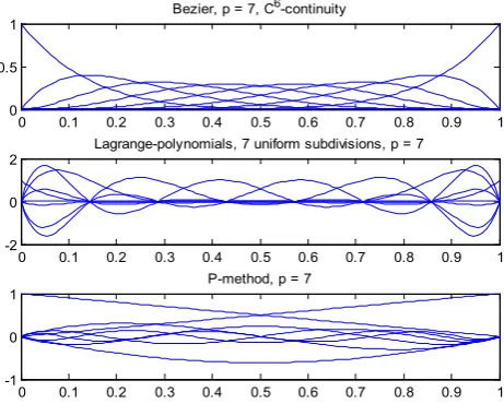
As one can notice in Fig.1, while Lagrange polynomials may exceed the unity and be characterized by high values particularly in the neighbourhood of the ends, Bernstein polynomials (or even general B-splines, not shown) are always less than or equal to unity (at the end nodes). It is worth-mentioning that, in both cases, the sum of the shape functions is equal to unity (rigid-body property, partition of unity). Similarly, in the p-method the sum of the first and last basis functions (N1 and N2, associated to the ends of the

domain) is equal to unity, whereas the intermediate “bubble functions”,

φ

_j, vanish at the ends but their sum is different than zero at every internal point (see, [21]).

A side ascertainment on the equivalency between the three functional sets in power series, i.e. Lagrange polynomials, Bernstein polynomials and the p-method is the numerical finding that the calculated eigenvalues are identical [32, 33]. 2.3. Two-Dimensional (2D) Interpolation

In brief, surfaces are categorized into quadrilateral and triangular patches, i.e. with four and three sides, respectively. The interpolations can treat either straight or curvilinear sides of the patch. The oldest way to create a 2D patch is Coons interpolation [1]. Later, tensor products of Bézier, B-splines and NURBS were applied [19, 27].

2.3.1. Quadrilateral Patches

[image:6.595.318.549.542.727.2]

We distinguish two categories. The first deals with data along the four boundaries of the quadrilateral; in other words, it consists the “boundary-only” formulation with nodal points along the boundary only. The second formulation uses the aforementioned boundary data as well as additional data in the interior of the quadrilateral; therefore it includes internal nodes as well, and is called “transfinite” interpolation.

Figure 1. Comparison between three equivalent sets of basis functions for seven uniform subdivisions using: (i) Bernstein (Bézier) polynomials, (ii)

0 0.1 0.2 0.3 0.4 0.5 0.6 0.7 0.8 0.9 1 0

0.5

1 Bezier, p = 7, C 6_-continuity

0 0.1 0.2 0.3 0.4 0.5 0.6 0.7 0.8 0.9 1 -2

0

2 Lagrange-polynomials, 7 uniform subdivisions, p = 7

0 0.1 0.2 0.3 0.4 0.5 0.6 0.7 0.8 0.9 1 -1

0

Lagrange polynomials, and (iii) p-method

2.3.1.1. Coons Interpolation

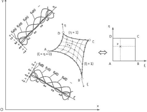
[image:7.595.62.308.181.376.2]

A four-sided region ABCD, as shown on the left of Fig.2, can easily be mapped to a unit square in the

ξη

parametric domain shown on the right of the same figure by the method of Coons’ patch [1]. For purposes of generalization, the relevant theory is given below using suitable projections.

Figure 2. Definition of the Coons-patch macroelement ABCD

First, the concept of the lofting projector ‘P’ is introduced. This projector is any idempotent linear operator, which maps a true surface to an approximate surface, subject to certain interpolatory constraints.

Let us assume that the Cartesian co-ordinates

(

,

) {

, ,

}

T

x y z

ξ η

=

x in A, with ξ and η denoting

normalized co-ordinates, are known at the boundaries (ξ =0,1; η=0,1) of a curvilinear patch of area A. Let us also define the well-known cardinal blending functions:

( )

( )

( )

( )

0 1 , 1 , 0 1 , 1

E ξ = −ξ E ξ =ξ E η = −η E η =η(26) Now, the following unidirectional, or lofting, operators

{ }

P

ξ

x

and

P

η

{ }

x

may be constructed (summation over repeated indices is understood):

{ } (

) ( )

{ } (

) ( )

,

,

,

.

i i

i i

P

E

P

E

ξ η

ξ η

ξ

ξ η

η

=

⋅

=

⋅

x

x

x

x

(27)

The above lofting operators form the basis for the definition of more complex operators with blending interpolation properties in more than one direction. So, the two-dimensional lofting operator:

{ }

{ }

(

_i

,

_j

)

_i

( )

_j

( )

P

ξη

x

=

P P

ξ η

x

=

x

ξ η

⋅

E

ξ

⋅

E

η

(28)

can be constructed with the aid of the unidirectional operators Pξ

{ }

x and Pη

{ }

x .

Finally, the co-ordinates of any point in the interior of the curvilinear patch is approximated as:

(

ξ η

,

)

=

(

P P P

_ξ

+

_η

−

_ξη

)

{ }

x

x

(29)

or, using conventional notation, as:

(

) (

) ( )

( )

(

) ( )

( )

(

)(

) ( ) (

) ( )

( ) (

) ( )

, 1 0, 1,

1 , 0 ,1

1 1 0, 0 1 1, 0

1 1 0

,1 ,1

ξ η ξ η ξ η

η ξ η ξ

ξ η ξ η

ξη ξ η

= − +

+ − +

− − − − −

− − −

x x x

x x

x x

x x

(30)

2.3.1.2. Gordon Interpolation

According to Gordon’s interpolation formula [34], the Cartesian coordinates

(

,

)

[

(

, ,

) (

,

)

]

T

x y

ξ η = ξ η ξ η

x of

each point P of in the patch can be approximated by its boundaries

(

x

(

ξ, 0 ,

) ( ) (

x ξ,1 ,x 0,η

) ( )

, 1,x η

)

as well as by its inter-boundaries (if any) as follows:

(

ξ η,

)

=Pξ

( )

+Pη

( )

−Pξη

( )

x x x x (31)

and

(

ξ η,

)

=Pξ

( )

+Pη

( )

−Pξη

( )

u u u u (32)

For example, based on Gordon’s interpolation, it is easy to derive the shape functions for a five-node element having one internal noded at its centre (in addition to the four ones at the corners) [35, 36].

Remark: It has been found that when the nodal points on the opposite sides of a patch possess identical normalized positions with those nodes in the interior, then Gordon-Coons interpolation degenerates to the cross product

P

ξη [37, p.328]. Under the latter conditions, when Lagrange

polynomials have been used, Coons interpolation coincides with the well-known interpolation in finite elements of Lagrange type (or Lagrange family) [5, p.153]. In conclusion, in patches where structured meshes of nodal points are used, all three basic CAD interpolations (Coons, Bézier, and B-splines) are expressed by a tensor product of 1-D ξ- and η-interpolations. Details are given below.

Figure 3. Definition of the Gordon-Coons macroelement ABCD

2.3.1.3. Tensor Products

[image:7.595.313.552.520.702.2]

curvilinear quadrilateral ABCD or a box-like volume ABCDEFGH, for a certain polynomial degree (p) and for a certain multiplicity (usually one or two), the basis functions

( )

,

i p

N

u

are determined. It is noted that here u is either of the normalized coordinates ξ, η, or ζ, whereas the number of basis functions equal to the (m+1) control points in the particular direction (mξ, mη, and mζ, in the ξ-, η-, or ζ-direction, respectively). Then, the aforementioned one-dimensional control points produce n = (1 + mξ)×(1 + mη)

or n = (1 + mξ)×(1 + mη)×(1 + mζ) control points for 2D and

3D problems, respectively. Each of the aforementioned control point is associated with one global shape function given by:

( )

( )

( )

( )

( )

for 2D problems for 3D problems ,

,

ip jp

I

ip jp kp

N N

N

N N N

ξ η

ξ η ζ

⋅ =

⋅ ⋅







(33)

Therefore, the geometry is interpolated by the expressions:

( )

( )

( )

( )

( )

( )

1 1 1

, , ,

, , ,

, , .

n

I I

I n

I I

I n

I I

I

x N x

y N y

z N z

ξ η

ξ η

ξ η

ξ η

ξ η

ξ η

=

=

= =

=

=

∑

∑

∑

(34)

2.3.1. Triangular Patches

We will present two alternatives as follows. 2.3.1.1. Side Degeneration

One possibility is to use the formulas previously used in quadrilateral patches, by degenerating one of the four sides into one point [1, p.3]. For example, when degenerating the entire side AD into a unique point A, the quadrilateral degenerates into a triangle ABC, (30) becomes [38, p.325]:

(

)

( )

( ) (

)

( )

[

(

)

]

,

1

1

BC AB

AC B C

u

u

u

u

u

u

ξ η

η ξ

ξ

η

ξ η ξ

η

η

=

⋅ +

⋅ −

+

⋅ −

−

+

(35)

2.3.1.2. Barnhill’s Formula

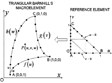
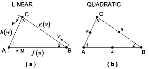
The mathematical description of triangular patches has been published by Barnhill [39-41]. In those works a “trilinearly blended interpolant” formulation is introduced, which is quite different than Gordon-Coons; today this formula can be found even in CAD textbooks such as [42, p.244]. The triangular patch shown in Fig. 4a can be mapped into the parametric patch of Fig. 4b through the relationship:

(

)

( )

(

)

( )

(

)

( )

(

)

( )

( )

( )

]

1 1

, ,

2 1 1 1

1 1

1 1 1

0 0 0

u g v wh v vh w P u v w

v v w

u f w w f u vg u

w u u

wf ug vh

−

= + +

− − −

− −

+ + +

− − −

− − −

 

(36)

The parametric patch of (36) is expressed as:

1 0

1, 0

1, 0

1

u v w

+ + =

≤ ≤

u

≤ ≤

v

≤ ≤

w

₍₃₇₎

In this case, the parametric patch can be intersected with increasing values of the variables u,v that vary between 0 and 1, and then calculating the corresponding values of w from each set of u and v.

[image:8.595.313.552.264.442.2]

Apart from CAD applications, no application of Barnhill’s formula to engineering analysis has been reported so far. For the first time, it is shown that, (36) inherently includes the conventional three- and six-nodedtriangular finite elements. Details are given in Appendix A and Appendix B, respectively. Of course, (36) allows for the derivation of novel arbitrary-noded triangular macroelements, that have been successfully applied to stress analysis problems [90].

Figure 4. Definition of the triangular parametric Barnhill’s patch

2.4. Three-Dimensional (3D) Interpolation

Volume blocks are categorized into hexahedral (eight vertices, and twelve edges) and tetrahedral (four vertices, and six edges) blocks. The interpolations can treat either straight or curvilinear edges of the volume.

2.4.1. General

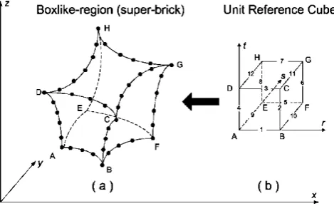
A boxlike region ABCDEFGH, shown in Fig. 5a, can easily be mapped to a unit cube in the rts parametric domain (0 ≤r,s,t≤ 1) shown in Fig. 5b. The relevant formula may be found in [1, p.41] and, as previously mentioned, is has been applied by Cook [43] for finite element mesh generation purposes. For more details the interested reader may also consult a textbook [44]. The only difference with a quadrilateral patch is that, here, six functions (associated to the six faces) are blended, instead of four functions (associated to the four boundary edges of the 2D patch). Below, the same formula is written in terms of projections.

Besides the above-mentioned Pr

{ }

x , Ps

{ }

x and

{ }

rs

follows:

{ }

(

)

( )

{ }

{ }

(

)

( )

( )

{ }

{ }

(

) ( )

( )

{ }

{ }

(

)

( )

( )

( )

, , , , , , , ,

t k k

st s t j k j k

rt r t i k i k

rst r s t i j k i j k

P r s t E t

P P P r s t E s E t P P P r s t E r E t

P P P P r s t E r E s E t

= ⋅

= = ⋅ ⋅

= = ⋅ ⋅

= = ⋅ ⋅ ⋅

x x

x x x

x x x

x x x

(38)

[image:9.595.60.295.222.370.2]

Again, summation over repeated indices is understood. Having introduced the one-, two- and three-dimensional operators, then the following formula describes the interpolation of the co-ordinate vector [1,p.41]:

Figure 5. Three-dimensional superbrick macroelement analyzed using “boundary-only” Coons formulation

(

)

( ) (

){ }

( ) (

){ }

( )

{ }

1 2 3

, , 1

1

1 .

r s t

rs st st

rst

r s t P P P

P P P P = − − ⋅ + + − − ⋅ + + − − ⋅ x x x x (39)

2.4.2. Equivalent Expressions of Trivariate Coons’ Formula 2.4.2.1. General Remarks

Equation (39) is generally applicable but it can be further simplified and be written in more readable expressions. So, in the case of a generalized curvilinear hexahedral /paralleloid (boxlike region), the geometry includes:

 Six surfaces, S  Twelve edges, E, and  Eight corners, C

Obviously, (39)includes all three quantities: Surfaces (S), edges (E) and corners (C). For convenience, the projections related to the S, E and C are denoted as follows:

{ } (

){ }

{ } (

){ }

{ }

x

{ }

x .

x x x x rst tr st rs t s r P C P P P E P P P S = + + = + + = (40)

However, in the case of adequately smooth and regular surfaces, the edges E can sufficiently describe S. In fact, applying (31) on the six surfaces of the superbrick, one can easily derive the following relationship:

{ }

x

C

{ }

x

E

{ }

x

S

+

3

=

2

(41)

Then, substituting (40) and (41) into (39), one can finally derive three equivalent expressions of the three-dimensional Coons’ interpolation formula, as follows:

(

) { } { } { }

x

x

x

x

r

,

s

,

t

=

S

−

E

+

C

(42)

(

)

{ }

x

{ }

x

x

r

,

s

,

t

=

1

2

S

−

1

2

C

(43)

(

)

{ }

x

{ }

x

x

r

,

s

,

t

=

E

−

2

C

(44) 2.4.2.2. Comments on 3D Equivalent Expressions

[image:9.595.313.553.325.444.2]

Obviously, (42) is the most general expression because it includes any type of the surrounding surfaces S (edge-only noded and/or internally noded). Moreover, (43) is obtained by eliminating the edges (E) and it is based on the surface S, the last being corrected by the co-ordinates of the corners C. Finally, (44)includes only the twelve edges E and eight corners C, or in other words, the absolutely necessary data for the construction of a Coons’ block made of Coons’ surfaces; it is evident that (44) uses nodal points arranged along the twelve edges only.

Figure 6. Overall applicability of Coons-interpolation

In conclusion, in cases where the superbrick is sufficiently regular, (44) is the most advantageous. Using conventional notation, (44) becomes:

(

) (

)( ) (

) (

) (

)

(

) (

) (

)(

) (

)

( ) (

)

( )

( ) (

) (

)

(

)( ) (

) (

) (

)

( ) (

)

(

)

(

)(

)( ) (

) (

)(

) (

)

[

(

) ( ) (

) (

)

(

)

(

)( ) (

) (

) (

)

(

1

)( ) (

1 ,1,10

)

( )

11,1,

]

1, 0 ,1 1 0 , 0 ,1 1 1 1, 1, 0 1 0 ,1 , 0 1 1 1, 0 , 0 1 1 0 , 0 , 0 1 1 1 2 1, ,1 0 , ,1 1 1, , 0 1 0 , , 0 1 1 ,1 , 0 1 1, 1, ,1 ,1 0 ,1 , 1 , 0 , 0 1 1 1, 0 , 1 , 0 ,1 1 0 , 0 , 1 1 , , x x x x x x x x x x x x x x x x x x x x x t s r t s r t s r t s r t s r t s r t s r t s r s t r s t r s t r s t r t s r r t s t s r r t s t s r r t s t s r r t s t s r + − − + − + − − + − + − − + − − + − − − − + − + − + − − + − + + + − + − − + − + − + − − = (45)

2.4.3. The Three Alternative Uses of Coons Interpolation In more detail, bivariate (2D) Coons interpolation on curvilinear surfaces is useful for (i) mesh generation for two different purposes (2D FEM or 3D BEM applications), and (ii) to derive 2D finite macroelements.

It has been previously reported that, the mesh produced by 2D-Coons interpolation can be easily smoothed by taking the average of the eight neighbouring nodes. Also, the mesh produced by 3D-Coons interpolation can be easily smoothened by taking the average of the twenty-six neighbouring nodes [45-47].

3. Use of Coons’ Interpolation

3.1. Older Findings

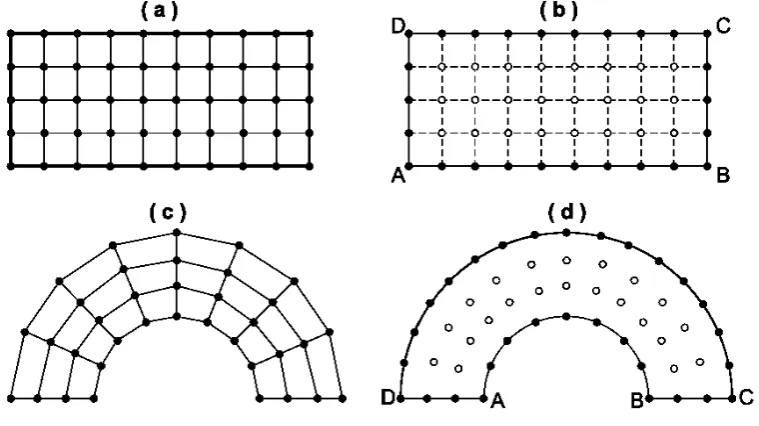
From the analysis sited in Section 2, it becomes clear that in 1967 Coons’ interpolation was the first achievement in CAD surface theory, primarily aiming at describing surfaces or volumes [1]. In early 1970s, FEM analysts understood that the same interpolation might have a second usage, as a generator of structured finite element meshes [43, 48-54]. In more details, first a mesh generation is constructed on the parent unit square or cube for 2D and D problems, respectively. Second, nodal points are constructed along the boundaries of the virtual structure. Third, (30), or (39) and its variations, are applied and thus establish a mapping between the aforementioned nodes in the parent element and the virtual structure. As a result, the desired finite element mesh is generated.

Moreover, it was early understood that Coons interpolation could be used for engineering analysis purposes as well [55, 56].

3.2. Contemporary Findings

3.2.1. Contribution on Conventional Finite Element Meshes In subsection 2.4.3 we mentioned that, due to the fact that the mesh generated using (30) or (39) for 2D and 3D problems, respectively, is usually of low quality, smoothing schemes have been successfully applied [57, 45-47]. The convergence leads to almost rectangular elements.

3.2.2. Construction of Gordon-Coons Macroelements for Engineering Analysis

3.2.2.1. Literature Survey

Early thoughts on the construction of large elements were made by the pioneer Bruce Irons [58]. Expressions of lower order large elements based on Coons-Gordon ideas are [55, 59-61]. Numerical examples on 2D potential problems were presented in 1989 by Kanarachos and Deriziotis [62] at the National Technical University of Athens (NTUA); as a member of NTUA’s FEM/BEM group, the author can confirm that relevant attempts started therein in 1982. This work was extended to 2D elasticity [63]; in the relevant conference the author announced that the same methodology is not applicable only to Coons but also in conjunction with all other CAD formulations such as Gordon-Coons, Bézier, B-splines and NURBS.

Boundary-only Coons interpolation was applied to 2D

potential problems [37, 64-68], axisymmetric elastostatics [69], and 2D elastodynamics [70-73]. In the process of the research it was found that boundary-only Coons interpolation corresponds to a series expansion of the solution with those terms appearing in Pascal’s triangle with a surplus of two (Serendipity family), a fact that was later found as a note in [74].

In some examples, the boundary-only Coons formulation was more accurate not only than the conventional FEM, with the same mesh density, but also than BEM [75].

It was later understood that, it is not always possible to accurately solve all engineering problems unless a sufficient number of internal nodes are used. The latter is easily achieved using Gordon-Coons (transfinite) interpolation [35-37, 72, 76]. Boundary-only Coons interpolation was successfully applied to 3D potential and elasticity problems [77-79]. The theme definitely closes with [80], which compares twelve alternative models one another; although it focuses on 2D elastostatics, the conclusions are of general importance.

Concerning BEM and solid modeling, initial attempts for CAD/CAE integration were made by Casale [81-83]. Application of Coons interpolation in 3D BEM problems was presented during the years 2001-2003 [84-87]; in these conferences the general applicability in conjunction with Bézier, B-splines and NURBS was repeated.

The overall conclusion is that boundary-only formulation sometimes cannot converge to the accurate solution, whereas the Gordon-Coons [88] always achieves it [89].

Concerning structures of triangular shape, the work of Kanarachos and Dimitriou [38, 89] has shown reliable results when a side of the quadrilateral is degenerated. In addition to the latter works, Provatidis and Antoniou [90] have found encouraging results when Barnhill’s interpolation [39-41] is used for the engineering analysis.

As one can see inspecting [91-109], Pierre Bézier was an employee of Renault (in France) and started publishing since 1966, which is almost the same period in which Steven Coons was working at MIT (in USA). Bézier’s theory is related to the discovery of the “control points”, which are vertices of a polygon (generator) that controls a curve. The same theory is also extended to curved surfaces, using a set of generators [19, 27]. Extension to volumes is possible [110]. In the context of engineering analysis, it has been found that Bézier formulation is equivalent to the use of monomials or Lagrange polynomials [111], a matter that has been also treated in 1D problems [32, 33, 112].

representation of circles requires rational degree two Bézier curves. Rational Bézier curves permit some additional shape control: by changing the weights, you change the shape of the curve. It is possible to reparametrize the curve by simply changing the weights in a specific manner.

Finally, in the process of CAD evolution, the use of B-Splines was proposed in 1973-1974 [116,117]. It is reminded that B-splines is nothing different than usual splines but they are replaced by non-cardinal basis functions,

( )

.

i p

N

ξ

of polynomial degree p, which are calculated for every normalized coordinate,

ξ

, through fast iterative formulas developed independently by Cox [29] and DeBoor [30] in 1972, as mentioned by the latter researcher in his monograph [26]. B-splines appear a local support and include, as a special case, the abovementioned Bézier curves. Despite the local support of B-splines, a better control on regional changes is achieved when using the non-uniform rational B-splines (NURBS) that were developed in mid-seventies till early eighties [118,119]. The interested reader may also consult a later survey [120] and a useful monograph of 646 pages [27].

According to the abovementioned sequence in CAD evolution, i.e. Gordon-Coons Bézier B-splines NURBS, a relevant contribution in structural (generally in engineering) analysis is anticipated, as follows. The common characteristic of all relevant works in engineering analysis is that, they all aim at decomposing the domain into CAD-controlled subregions [121-124].

Concerning Gordon-Coons (transfinite) interpolation, relevant research on graphics continued at least until 2004 [125-128], whereas engineering analysis was made in electrical engineering [129] and soft-tissue biomechanical [130] applications. Initial works are [55, 59-61]. As regards the FEM/BEM group at NTUA, isoparametric Gordon-Coons macroelements were published in the period 1989-2011 [38, 57, 62-73, 75-80, 84-90].

In this paper we will use the term “isogeometric” when referring to interpolations related to “control points”, i.e. Bézier, B-splines and NURBS.

Concerning Bézier representation, it is reminded that it is equivalent with the use of Lagrange polynomials [111]. In other words, for any selected degree of the polynomials involved, despite the fact that the control points sweep the entire domain, in fact it is “as if nodal points along only the sides”were used (2D: 4 sides of the quadrilateral, 3D: 12 edges of the hexahedron).

Concerning B-splines in engineering analysis, a forgotten but (in author’s opinion) pioneering work is due to Aristodemo [131] and later a lot of papers appeared [132-141]. Among these works, [137-141] refer to the boundary element method (BEM).

Concerning the evolution in NURBS, the interested reader may consult [142], among others. One of the first attempts to incorporate NURBS in structural analysis, and particularly in shape optimization, is due to Schramm and Pilkey [143], in 1993, followed by other investigators such as [144-146]. In 2005, the group of Prof. T. J. R. Hughes introduced the term

“isogeometric” elements [147-149], and later they applied an efficient quadrature to reduce the CPU-time [150].

The author [68] had timely discovered that, despite its elegance, the global interpolation is generally slower than the common finite element method (Galerkn-Ritz), of course for the same mesh density. In 2005, he proposed to preserve the CAD-based global interpolation and replace the domain integration through a global collocation scheme [73, p. 6704].

Concerning the Global Collocation Method (GCM), an initial contribution is due to Blerk and Botha [151]. The problem was systematically tackled starting from one-dimensional problems, first starting with Lagrange polynomials [22, 23, 152] and then continuing with B-splines [153, 154]. Then, the same idea was extended to 2D potential problems [155, 156], elastostatics [157], as well as eigenvalue problems in acoustics and elastodynamics [158, 159]. It is worth-mentioning that the application of isogeometric collocation methods was later proposed by others [160].

3.2.2.2. Global Shape Functions

Following [80], let us assume that the sides AB, BC, CD and DA of the patch ABCD shown in Fig. 3 include q1, q2, q3

and q4 nodes, respectively. In this case, the corresponding

number of subdivisions per side are n1=q1-1, n2=q2-1,

n3=q3-1 and n4=q4-1, respectively. Then, the number of

nodes along the boundary of the patch becomes:

1 2 3 4 1 2 3 4 4

b

q =n n+ +n +n =q q+ +q +q − (46) while considering the additional

n

_I internal nodes, the total number of nodes becomes:

I

e b

q =q +n (47) In the sequence, the boundary values of the displacement vector, i.e. u(ξ,0), u(1,η), u(ξ,1) and u(0,η) in (30) or finally in (32), are interpolated by any set of basis functions

( )

ˆ

j

B

ξ

like those presented in Section 2 (

ξ

ˆ is either ξ or η ; the upper index in Bj below corresponds to the relevant side

of the Coons patch):

( )

( )

( )

( )

( )

( )

( )

( )

( )

( )

( )

(

)

1

2

3

4

AB

1

BC

1

CD

1

DA

1

AB:

,0

,0

Side BC:

1,

1,

Side CD:

,1

,1

Side DA:

0,

0,

Side

q j j

j q

j j

j q

j j

j q

j j

j

B

B

B

B

ξ

ξ

ξ

η

η

η

ξ

ξ

ξ

η

η

η

= = = =

=

=

=

=

∑

∑

∑

∑

u

u

u

u

u

u

u

u

(48)