Note on Transportation Problem with New Method for Resolution of Degeneracy

Note on Transportation Problem with New Method for

Resolution of Degeneracy

Sarbjit Singh

Institute of Management Technology, Nagpur, India

Copyright © 2015 Horizon Research Publishing All rights reserved.

Abstract

Transportation algorithm minimizes the cost of transporting goods from m origins to n destinations along m*n direct routes from origin to destination. There are three methods to solve transportation problem and their solution can be further improved using Modified Distribution Method (MODI Method). This method not only checks that the solution obtained by three methods is optimal but also modify the distribution to make it optimal. The only hiccup with this method is the case of degeneracy i.e. when number of allocations less than m+n-1. In this case, we have to make the number of allocations equal to m+n-1. To remove degeneracy we allocate some cells with dummy allocations, whose value is nearly equal to zero. But, till now there is no specific rule for allocating these cells. In this study, specific method has been proposed to remove this problem of degeneracy. Thus this study helps to remove major bottle neck from transportation algorithm.

Keywords Transportation Problem, Degeneracy,

Modified Distribution Method, Vogel Method, Least Cost Method

1. Introduction

Transportation theory is a name given to the study of optimal transportation and allocation of resources. The problem was formalized by the French mathematician Gaspard Monge(1871). In the 1920s A.N. Tolstoi was one of the first to study the transportation problem mathematically. In 1930, in the collection Transportation Planning Volume I

for the National Commissariat of Transportation of the Soviet Union, he published a paper Methods of Finding the Minimal Kilometrage in Cargo-transportation in space. Tolstoi(1939) illuminated his approach by applications to the transportation of salt, cement, and other cargo between sources and destinations along the railway network of the Soviet Union. In particular, a, for that large-scale, instance of the transportation problem was solved to optimality.

Major advances in transportation theory were made in the field during World War II by the Soviet/Russian

mathematician and economist Leonid Kantorovich Consequently, the problem as it is stated is sometimes known as the Monge–Kantorovich transportation problem. Kantorovich won the Nobel prize for economics in 1975 for his work on the optimal allocation of scarce resources, the only winner of the prestigious award to come from the USSR.

F.L. Hitchcock (1941) worked on the distribution of a production from several sources to numerous localities. Koopman also worked on the optimum utilization of transportation system and used model of transportation, in activity analysis of production and allocation.

Charnes and Cooper (1961) mentioned about transportation in their book – Management Models and Industrial Applications of Linear Programming. Followed by Ijiri (1965) who mentioned about transportation problem in his book- Management Goals and Accounting for Control

M. Klein (1967) developed a primal method for minimal cash flows with applications to the assignment and transportation problems. Hadley(1972) also included transportation problem in his book: Linear Programming. Lee (1972) and Ignizio(1976) used goal programming to solve transportation problem.

Mackinnon & James (1975) developed an algorithm for the generalized transportation problem. Moore et-al performed analysis of a transshipment problem with multiple conflicting objectives. Kwak (1979) developed a goal programming model for improved transportation problem solutions, followed by Kvanli (1980).

OhEigeartaigh (1982) developed a fuzzy transportation algorithm Arthur-et-al (1982) worked on the multiple goal production and logistics planning in a chemical and pharmaceutical company. Olson (1984) has compared four goal programming algorithm. Goyal(1984) worked on improving VAM for unbalanced transportation problem.

Romero (1991) has written a book on critical issues in goal programming, followed by Tamiz & Jones (1995) who has done a review of goal programming and its applications. Hemaida & Kwak(1994) developed a linear goal programming model for transshipment problem with flexible supply and demand constraints. Sharma et-al (1999) analyzed various applications of multi-objective programming in MS/OR.

Sun (2002) worked on the transportation problem with exclusionary side constraints and branch and bound algorithm. Schrijver(2002) worked on the history of transportation and maximum flows. Okunbor(2004) worked on the management decision making for transportation problems through goal programming.

In this study, for resolution of degeneracy method has been proposed. The problem of degeneracy can occur in initial solution or it may arise in some subsequent iterations. Transportation Problem

 The transportation Problem is one of the special type of Linear Programming Problem in which objective is to transport various quantities of single identical goods that are initially stored at various origins, to different destinations in such a way that the total transportation cost is least.

 Vogel’s Approximation Method is one of the most efficient methods to obtain basic feasible solution, which is most near to the optimal solution.

 Then usually we check the optimality of the solution with the help of either stepping stone method (Charnes and Cooper, 1954) or Modified Distribution (MODI) method.

 In order to check the optimality of the cost, we apply the optimality criteria: There must be (m+n-1) number of allocated cells (m-number of rows, n-number of columns). If the number of allocated cells is less than (m+n-1), then it is a degenerate Transportation Problem

 In this article we will propose a technique of resolving degeneracy, which is not given in text books.

 There are three methods of obtaining a feasible solution:

i. North West Corner Method (Layman’s Method)

ii. Least Cost Method (Business Man’s Method) iii. Vogel’s Approximation Method (Operations

Method)

Formulation of a General Transportation Problem

Consider that there are m sources Source1, Source2, …….., Source m with capacities

1

, ,...,

2 m

a a

a

and n-destinations (sinks) with requirements

b b

₁

, ,...,

₂

b

_m respectively. The transportation cost from ith source to jth destination is

c

_ij and the amount shipped is

x

_ij. If the total capacity of all sources is equal to the total requirement of all the destinations, what must be the values of

ij

x

with i=1,2,…..,n for the total transportation cost to be minimum?

Source/

Destination D1 D2 .. Dj .. Dn Availability

S1

c

₁₁

c

₁₂

c

_1j

c

_1n

a

₁

S2

c

₂₁

c

₂₂

c

2j

c

2n

a

2

: :

Si

c

_i1

c

_i2

c

_ij

c

_in

a

_i :

:

Sm

c

_m1

c

_m2

c

_mj

c

_mn

a

_m

Requirements

b

₁

b

₂

b

_j

b

_n

i

j

a

b

=

∑

The Mathematical formulation of the transportation problem is given by

Minimize

1 1

m n ij ij i j

z

c x

= =

=

∑∑

Subject to 1

1

, 1,2,....

, 1,2,....

n

ij i

j m

ij j

i

x

a i

m

x

b i

n

=

=

=

=

=

=

∑

∑

and

x

ij

≥

0

for all i and j.

There are three methods to obtain the feasible solution a) North West Corner Method

b) Least Cost Method

c) Vogel’s Aprroximation Method

a) North West Corner Method

This method is also called layman’s method, as in this method the only motive is to have a balance between demand and supply. This is the oldest method known and had been in use, even before any of the method is known. We have to follow the following steps to solve the problem using this method.

Algorithm

Step 1: Locate the cell in the north-west (upper left) corner of the matrix of the data completely ignoring the transportation cost.

Step 2: Transport the minimum of demand and supply values with respect to that cell and subtract this minimum from the supply and demand values.

Step 3: Check whether exactly one of the row/column corresponding to the north-west corner cell has now zero supply/demand respectively or both of them has zero.

Step 4: Delete the row or column or both depending upon whichever is having zero

Step5: Repeat the steps 1-4 with the reduced matrix unless all demand and supply becomes zero

The gist of this method is to start transporting from first source to first factory and then whichever is possible i.e., either from first source to second destination or from source 2 to first destination depending upon the demand and supply. The process continues unless all the units are transported.

Problem 1

The Oberoi car company has warehouses in Amritsar (

W

₁), Nanded (

W

₂) and Patna (

W

₃) and markets in Noida (

M

₁), Bangalore (

M

₂), Kolkata (

M

₃) and Gandhinagar (

M

₄)

Factory /

Markets

M

1

M

2

M

3

M

4 Availability 1

W

24 23 43 14 60

2

W

34 32 12 40 80 3

W

20 22 23 41 100 Demand 40 70 80 50 Total=240

Tables below explain the North West Corner Method Step1

Factory /

Markets

M

1

M

2

M

3

M

4 Availability 1

W

24(40) 23 43 14 20 2

W

32 12 40 80

3

W

22 23 41 100

Demand 70 80 50 Total=240

Step2

Factory /

Markets

M

1

M

2

M

3

M

4 Availability

1

W

24(40) 23(20) 2

W

32 12 40 80

3

W

22 23 41 100

Demand 50 80 50 Total=240

Step3

Factory /

Markets

M

1

M

2

M

3

M

4 Availability

1

W

24(40) 23(20) 2

W

32(50) 12(30) 3

W

23(50) 41(50)

Demand Total=240

The cost associated with this basic feasible solution is computed as follows

24*40+23*20+32*50+12*30+23*50+41*50=6580

b) Least cost Method

This method is also called Business man’s method, as in this case a business that is having no knowledge of operations management is considered. His only motive to reduce the transportation cost, while having a balance between demand and supply. He always tries to allocate items to the cells having minimum transportation cost.

Algorithm

Step 1: find the cell with minimum per unit transportation cost.

Step 2: Transport the minimum of demand and supply values with respect to that cell and subtract this minimum from the supply and demand values.

supply/demand respectively or both of them has zero. Step 4: Delete the row or column or both depending upon whichever is having zero

Step5: Repeat the steps 1-4 with the reduced matrix unless all demand and supply becomes zero

Consider Oberoi Car Company problem again using least cost method.

Tables below explain the Least Cost Method with problem1

Step1

Here least cost is 12, and we can assign 80 units there

Factory /

Markets

M

1

M

2

M

3

M

4 Availability

1

W

24 23 43 14 60

2

W

34 32 12(80) 40 80

3

W

20 22 23 41 100 Demand 40 70 80 50 Total=240

Step 2 Next minimum is 14 and we can assign 50 units there

Factory /

Markets

M

1

M

2

M

3

M

4 Availability

1

W

24 23 14(50) 10

2

W

12(80)

3

W

20 22 100

Demand 40 70 Total=240

Step 3 Next minimum is 20 and we can assign 40 units there

Factory /

Markets

M

1

M

2

M

3

M

4 Availability

1

W

23 14(50) 10

2

W

32 12(80)

3

W

20(40) 22 60

Demand 70 Total=240

Step 4 Next minimum is 22 and we can assign 60 there and remaining 10 to 23

Factory /

Markets

M

1

M

2

M

3

M

4 Availability

1

W

23(10) 14(50)

2

W

12(80)

3

W

20(40) 22(60)

Demand Total=240

The total transportation cost is

23*10+14*50+12*80+20*40+22*60=4010

As it can be observed that the total cost obtained by this

method is very less than the total cost obtained by North West Corner method. The major disadvantage with North West Corner method is that cost does not play any role in that method. The only aim of using that method is to a balance between demand and supply.

The disadvantage with this method is that finally we have to transport some of the items with very high cost

c) Vogel’s Approximation Method (VAM)

This method is also known as penalty method. This method is based upon the concept that if you miss best (lowest cost) in first attempt you have to face the penalty in next attempt. Hence, for each source and destination, we compute a ‘penalty’ rating which is the difference in cost of the two cheapest routes for the source and destinations. The major advantage of this method is solution given by this method is closer to the optimal solution.

Algorithm

Step 1: From the transportation table, we determine the penalty for each row and column. The penalties are calculated for each row (or column) by subtracting the lowest cost element in that row (column) from the next lowest cost element in the same row (column). Write down the penalties below the rows (aside the columns) of the table. Step 2: Select the row (column) with the highest penalty rating and allocate as much as possible from the supply and requirement values to the cell having the minimum cost. If there is a tie in the values of penalties, then check the next level penalty i.e., the next two minimum cost, the route having more next penalty will be chosen. (New Rule for a tie of penalties)

This rule is extremely helpful in obtaining basic feasible solution in close proximity to the optimal solution

Step 3: Adjust the supply and demand conditions for that cell. Eliminate those rows (columns) for which the supply and demand requirements are met.

Step 4: Repeat the steps 1-3 with the reduced table unless all demand and supply becomes zero

Thus, we obtain an initial basic feasible solution.

Tables below explain the Vogel Approximation Method with problem1

Step 1

Factory /

Markets

M

1

M

2

M

3

M

4 Availability Penalty

1

W

24 23 43 14(50) 10 9

2

W

34 32 12 80 20

3

W

20 22 23 100 2

Demand 40 70 80

Step 2

Factory /

Markets

M

1

M

2

M

3

M

4 Availability Penalty

1

W

24 23 14(50) 10 9 2

W

12(80) 20

←

3

W

20 22 100 2

Demand 40 70 Penalty 4 1 9

Step 3

Factory /

Markets

M

1

M

2

M

3

M

4 Availability Penalty 1

W

23 14(50) 10 1

2

W

12(80)

3

W

20(40) 22 60 2

Demand 70 Penalty 4

↑

1

Step 4

Factory /

Markets

M

1

M

2

M

3

M

4 Availability Penalty 1

W

23(10) 14(50) 2

W

12(80)

3

W

20(40) 22(60) Demand

Penalty

The total transportation cost is

23*10+14*50+12*80+20*40+22*60=4010

From this cost it looks like that Vogel’s Approximation method as well as Least Cost Method is giving same basic feasible solution. But it is not true in most of the cases Vogel’s Approximation method gives better solution. Hence, we are considering one more example to show that VAM is better than Least Cost Method

Problem2

Solve the following transportation problem

To

From

1 2 3 Supply

1 2 7 4 5

2 3 3 1 8

3 5 4 7 7

4 1 6 2 14

Demand 7 9 18 34

Firstly we will solve this problem using Least Cost Method,

To

From

1 2 3 Supply 1 7(2) 4(3)

2 1(8)

3 4(7)

4 1(7) 2(7) Demand

The total Transportation cost is 7*2+4*3+1*8+4*7+2*7+1*7=83

The table below gives the basic feasible solution obtained by using Vogel’s Approximation Method

To

From

1 2 3 Supply 1 2(5)

2 3(2) 1(6)

3 4(7)

4 1(2) 2(12) Demand

The total Transportation cost is 2*5+3*2+1*6+4*7+1*2+2*12= 76

Hence, from above problem, we can conclude the basic feasible solution obtained from Vogel’s Approximation is better Least Cost Method.

Modified Distribution Method

The basic feasible solution obtained by above methods are not necessarily optimal, therefore, we have to check the optimality of the above solution. The most reliable method to check the optimality of the basic feasible solution is Modified Distribution Method (MODI Method)

It’s a fact that solution obtained by VAM is more nearer to optimal solution than any other method. The necessary condition for applying this method is there must be m+n-1 allocations; otherwise it is a case of degeneracy, which we discuss later on.

Algorithm

Step 1: We find the initial basic feasible solution by applying any of the above methods, preferably with VAM on a balanced transportation problem.

Step 2: Assign variables

u

_iand

v

_j to each row and columns. Then

u

_ior

v

_jshould be taken as zero, for which maximum number of allocations are made in its row or column.

Step 3: For allocated cells, we divide the cost as

j i ij

u

v

c

=

+

Step 4: Examine the sign for each

∆

_ij

ii) If some

∆

_ij

≤

0

,

then the cost obtained is not optimal. It has to be reduced by some technique (given in next step).

Step 5: In the cell having the most negative value of

∆

_ij, we will make allocations. Rescheduling of allocations is done by the looping process.

Find the closed path with the selected unoccupied cell and allocate an unknown quantity

ϑ

, to the cell. Add and subtract interchangeably,

ϑ

to and from the transition cells of the loop in such a way that the rim requirements remain satisfied.

Firstly we will take a solution obtained by least cost method and check its optimality, as we know the solution obtained by this method; it helps us to learn the whole algorithm

Step1

(2) (3) (-1) (7) 2 (4) 3

u

₁=4

(3) (2) (1) (3) (4) (-1) (1) 8

u

₂=1

(5) (0) (5) (4) 7 (7) (1)

u

₃=1

(1) 7 (6) (5) (2) 7

u

₄=2

1

v

=-1

v

₂=3

v

₃=0

As two

∆

_ij are negative, hence solution obtained is not optimal. Thus, we modify the distribution of allocation to make the solution optimal. The thumb rule says we must select the most negative, but as here both are having same negative value, so we can take any one of them

Step 2

(2) (-1) (7) 2-2 (4) 3+2

(3) (1) (3) 2 (-1) (1) 8-2

(5) (5) (4) 7 (7)

(1) 7 (6) (2) 7

Now total cost = 3*2 +4*5+4*7+1*6+1*7+2*7=81, which has reduced by 2 units

Step 3

(2) (3) (-1) (7) (5) (2) (4) 5

u

1=4

(3) (0) (3) (3) 2 (1) 6

u

2=1

(5) (1) (4) (4) 7 (7) (2) (5)

u

3=2

(1) 7 (6) (3) (3) (2) 7

u

4=2

1

v

=-1

v

₂=1

v

₃=0

Again one

∆

_ij is negative; hence solution obtained is not optimal. Thus, we modify the distribution of allocation to

make the solution optimal. Step 4

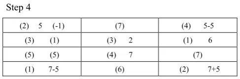
(2) 5 (-1) (7) (4) 5-5 (3) (1) (3) 2 (1) 6 (5) (5) (4) 7 (7) (1) 7-5 (6) (2) 7+5

Now total cost = 2*5+3*2+1*6+4*7+1*2+2*12=76, which has been reduced further by 5 units. This also the basic feasible solution obtained by VAM. Now we will check the optimality of this solution. As we have two rows and one column with 2 assignments we can choose any one of them

Step 5

(2) 5 (7) (5) (2) (4) (3) (1)

u

₁=2

(3) (0) (3) (3) 2 (1) 6

u

₂=0

(5) (1) (4) (4) 7 (7) (2) (5)

u

₃=1

(1) 2 (6) (4) (2) (2) 12

u

₄=1

1

v

=0

v

₂=3

v

₃=1

As all

∆

_ij are positive; hence solution obtained is optimal.

Special Case of Degeneracy Problem 3

There are three factories and they are supplying their goods to 4 markets, the cost matrix of the problem is given below. Obtain the optimal transportation cost.

Factory /

Markets

M

1

M

2

M

3

M

4 Availability

1

F

1 2 3 4 6

2

F

4 3 2 0 8

3

F

0 2 2 1 10

[image:6.595.310.554.95.175.2]

Demand 4 6 8 6 Total=24

Table below gives solution using Vogel’s Approximation Method for problem 3

Factory /

Markets

M

1

M

2

M

3

M

4 Availability 1

F

1 2(6) 3 4 6

2

F

4 3 2(2) 0(6) 8

3

F

0(4) 2 2(6) 1 10 Demand _{4 6 8 6 Total=24}

Minimum cost = 2*6 + 2*2 +0*6 +0*4+2*6=28

First we will follow the regular steps of MODI method, then the rows in which there are no allocations will be assigned a very small value

ε

₁ ,

ε

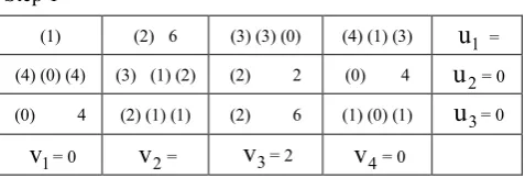
₂ etc, depending on the number of less allocations than m+n-1 . Most of the practical aspects we will not be having more than two less allocations

Step 1

(1) (2) 6 (3) (3) (0) (4) (1) (3)

u

₁ = (4) (0) (4) (3) (1) (2) (2) 2 (0) 4

u

₂= 0

(0) 4 (2) (1) (1) (2) 6 (1) (0) (1)

u

₃= 0

1

v

= 0

v

₂=

v

₃= 2

v

₄= 0

In this first step, on applying MODI’s method we are not able to get the value of

u

₁ , there for we will put

ε

in first row or second column and obtain the values of

u

₁ and

v

₂ Step 2

(1)

ε

(2) 6 (3) (3) (0) (4) (1) (3)

u

₁ = 1

(4) (0) (4) (3) (1) (2) (2) 2 (0) 4

u

₂= 0

(0) 4 (2) (1) (1) (2) 6 (1) (0) (1)

u

₃= 0

1

v

= 0

v

₂=1

v

₃= 2

v

₄= 0

In this way, we can easily resolve the problem of degeneracy in transportation problem. In my view it will help students in resolution of degeneracy in much easier way. In case of two less allocations similarly, we can put

ε

₁ ,

ε

₂ in rows or columns for which we are not getting the value of the variables.

The solution obtain in the above problem is optimal solution as all the differences obtained positive or zero, as one difference is zero, hence alternate optimal solution is

possible

Problem 4

Consider the case of five factories and five markets with per unit transportation cost

Factory/Market 1 2 3 4 5 Supply

1 80 69 103 64 61 12 2 47 100 72 65 40 16

3 16 103 87 36 94 20

4 86 15 57 19 25 8

5 27 20 72 94 19 8

[image:7.595.59.298.153.234.2]

Availability 16 14 18 6 10

Table below gives solution with Vogel’s Approximation Method

Factory/

Market 1 2 3 4 5 Supply 1 80 69 ₍₁₂₎ 103 64 61

2 47 100 ₍₆₎ 72 65 ₍₁₀₎ 40

3 ₍₁₆₎ 16 103 87 ₍₄₎ 36 94

4 86 ₍₆₎ 15 57 ₍₂₎ 19 25

5 27 ₍₈₎ 20 72 94 19 Availability

Which gives only eight allocations; hence it is the case of degeneracy

Tables below give the solution of problem 4 using MODI method.

Step 1

1 2 3 4 5

1 (80) (69) (103) (12) (64) (61)

u

₁=79

2 (47) _ε (100) (72) ₍₆₎ (65) ₍₁₀₎ 40

u

₂= 48

3 (16) ₍₁₆₎ (103) (87) (36) ₍₄₎ (94)

u

₃=17

4 (86) (15) ₍₆₎ (57) (19) ₍₂₎ (25)

u

₄= 0

5 (27) (20) ₍₈₎ (72) (94) (19)

u

₅=5

1

On applying MODI’s method both first and second row has not got any allocation. Putting εin second row having minimum cost in both the rows we obtain the following matrix.

Step 2

1 2 3 4 5

1 (80) (78) ₍₂₎ (69) (94) _(-25) (103) ₍₁₂₎ (64) (98) _(-34) (61) (71) _(-10)

u

₁=79

2 (47) _ε (100) (63) ₍₃₇₎ (72) (6) (65) (67) _{(-2) (10)} 40

u

₂= 48

3 (16) (16) (103) (32) ₍₇₁₎ (87) (41) ₍₄₆₎ (36) (4) (94) (9) ₍₈₅₎

u

₃=17

4 (86) (-1) ₍₈₇₎ (15) ₍₆₎ (57) (24) ₍₃₃₎ (19) (2) (25) (-8) ₍₃₃₎

u

₄= 0

5 (27) (4) ₍₂₃₎ (20) ₍₈₎ (72) (29) ₍₄₃₎ (94) (24) ₍₇₀₎ (19) (-3) ₍₂₂₎

u

₅=5

1

v

=-1

v

₂=15 v₃=24

v

₄=19

v

₅= -8

Step 3

Shifting εto the cell having most negative element in first row, and checking the optimality using Modified Distribution Method, we have

1 2 3 4 5

1 (80) (44) ₍₃₆₎ (69) (60) ₍₉₎ (103) ₍₁₂₎ (64) _{ε (-10)} (61) (71)

u

₁=0

2 (47) (13) ₍₃₄₎ (100) (29) ₍₆₁₎ (72) ₍₆₎ (65) (67) _{(-2) (10)} 40

u

₂= -31 3 ₍₁₆₎ (16) (103) (32) ₍₇₁₎ (87) (75) ₍₁₂₎ (36) ₍₄₎ (94) (43) ₍₅₁₎

u

₃= -28

4 ₍₈₇₎ (86) (-1) (15) ₍₆₎ (57) (58) _(-1) (19) ₍₂₎ (25) (26) _(-1)

u

₄= -45

5 ₍₂₃₎ (27) (4) (20) ₍₈₎ (72) (63) ₍₉₎ (94) (24) _{(70) (-12)} (19) (31)

u

₅=-40

1

v

=44

v

₂=60

v

₃=103

v

_{4= 64}

v

₅= 71

Step 4

Again modifying the distribution we obtain the reduced matrix with 9 allocations, hence degeneracy is resolved

1 2 3 4 5

1 (80) (44) ₍₃₆₎ (69) (72) _(-3) (103) ₍₁₀₎ (64) ₍₂₎ (61) (71) _(-10)

u

₁= 0

2 (47) (13) ₍₃₄₎ (100) (41) ₍₅₉₎ (72) ₍₈₎ (65) (33) ₍₃₂₎ (40) ₍₈₎

u

₂= -31

3 (16) ₍₁₆₎ (103) (34) ₍₆₉₎ (87) (75) ₍₁₂₎ (36) ₍₄₎ (94) (43) ₍₅₁₎

u

₃= -28

4 (86) (-13) ₍₉₉₎ (15) ₍₈₎ (57) (46) ₍₁₁₎ (19) (7) (25) (14) ₍₁₁₎

u

₄= -57

5 ₍₃₅₎ (27) (-8) (20) ₍₆₎ (72) (51) ₍₂₁₎ (94) (12) ₍₇₂₎ (19) ₍₂₎

u

₅= -52

1

Step 5

Again modify the distribution we obtained the following matrix

1 2 3 4 5

1 (80) (44) ₍₃₆₎ (69) (62) ₍₇₎ (103) ₍₂₎ (64) ₍₂₎ (61) (8)

u

₁= 0

2 (47) (13) ₍₃₄₎ (100) (31) _{(69) (16)} (72) (65) 33) ₍₃₂₎ (40) (30) ₍₁₀₎

u

₂= -31 3 (16) ₍₁₆₎ (103) (34) ₍₆₉₎ (87) (75) ₍₁₂₎ (36) ₍₄₎ (94) (33) ₍₆₁₎

u

₃= -28

4 (86) (-13) (99)

(15)

(8) (57) (56) (1) (19) (17) (2) (25) (14) (11)

u

4= -47

5 (27) (2) (25)

(20)

(6) (72) (61) (11) (94) (22) (72) (19) (2)

u

5= -42

1

v

=44

v

₂=62

v

₃=103

v

₄=64

v

₅=61

The solution obtain in the above problem is optimal solution as all the differences obtained positive, hence, the total transportation cost comes out to be $2652

Special Cases

a) Unbalanced Transportation problem. A necessary and sufficient condition for existence of feasible solution is that total demand must be equal to the total supply, i.e.

1 1

m n

i j

i j

a

b

= =

=

∑

∑

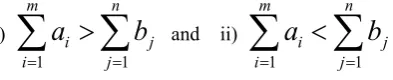
However, sometimes there may be more demand than the supply and vice versa in which case it is said to be unbalanced. It may occur in the following situations:

i)

1 1

m n

i j

i j

a

b

= =

>

∑

∑

and ii)

1 1

m n

i j

i j

a

b

= =

<

∑

∑

In case I, we introduce a dummy destination in the transportation table. The cost of transporting to this are all set equal to zero. The requirement at this dummy destination is then assumed to be equal to

1 1

m n

i j

i j

a

b

= =

−

∑ ∑

In case II, we introduce a dummy source in the transportation table. The cost of transporting from this source to any destination is all set equal to zero. The availability at this dummy source is assumed to be equal to

1 1

n m

j i

j i

b

a

= =

−

∑ ∑

b) Maximization Problem. In, general, transportation method is used for minimization problems. However, it can also be used to solve problem in which objective is to maximize when we consider the unit profit (or payoff)

p

_ij instead of unit cost

c

_ij

associated with route (i,j). The solution process to solve such problems is given below.

[image:9.595.60.257.469.509.2]

First, convert the given problem into minimization problem by replacing each element of the transportation table by its difference from the maximum element of the table.

Second, obtain an initial feasible solution using any of the three methods.

Third, use Modified Distribution Method for finding an optimal solution.

c) Prohibited Routes- The situation may arise such as road hazards (snow, flood, etc.), traffic regulations, strike etc., when it is not possible to transport goods from certain sources to certain destinations. Such type of problem can be handled by assigning infinite cost (∞) to that route (or cell)

d) Alternative optimal solutions- the existence of alternative optimal solutions can be determined by an inspection of the opportunity costs,

z

_ij

−

c

_ij for the unoccupied cells. If an unoccupied cells. If an unoccupied cell in an optimal solution has opportunity cost of zero, then an alternative optimal solution can be formed with another set of allocations without increasing the total transportation cost. To obtain an alternate solution, trace a closed loop beginning with cell having

∆

_ij=0, and get the revised solution in the same way as a solution is improved. It may be observed that this revised solution would also entail the same total cost as before. It goes without saying that for every ‘zero’ value of

∆

_ij value in the optimal solution tableau, a revised solution is obtained.

e) Assignment Problem- Assignment problem is a special case of transportation problem having equal number of sources and destinations (sink), and all

i

a

and

b

_jequal to one. Thus, assignment problem can also solve with the help transportation algorithm. f) Transshipment Problem- A transportation problem

units on the origins and destinations respectively. An m-origin, n-destination, transportation problem, when expressed as a transshipment problem, shall become an enlarged problem: with m + n origins and an equal number of destinations. With minor modification this problem can be solved using the transportation algorithm.

2. Conclusions

Transportation problem is one of most popular type of linear programming problem. The algorithm to get solution of transportation problem has been widely used to solve transportation problem in various cases. The only drawback with transportation problem is the case of degeneracy i.e. when numbers of allocations are less than m+n-1, there was no exact rule to resolve this degeneracy. In this study, a method is developed to resolve the problem of degeneracy. Hence, this study tries to make transportation algorithm more efficient and user friendly.

Appendix

Theorem 1 (Existence of a feasible solution)

The necessary and sufficient condition for the existence of a feasible solution to the Transportation Problem is

1 1

m n

i j

i j

a

b

= =

=

∑

∑

, that is, the total capacity (supply) must equal total requirement (demand)

Theorem 2

The dimensions of the basis of a Transportation Problem are (m+n-1) (m+n-1). This means that a Transportation problem has only (m+n-1)-independent structural constraints and its basic feasible solution has only (m+n-1)- positive components.

REFERENCES

[1] Ahuja, R.K.(1986). Algorithms for minimax transportation problem. Naval Research Logistics Quarterly.33 (4), 725-739.

[2] Arthur, J.L & Lawrence, K.D., (1982). Multiple goal production and logistics planning in a chemical and pharmaceutical company. Computers & Operations Research. 9(2), 127-137.

[3] Charnes, A. and Cooper, W. W. (1961). Management Models and Industrial Applications of Linear Programming, 1, John Wiley & Sons, New York

[4] Currin, D.C.(1986) Transportation problem with inadmissible routes. Journal of the Operational Research

Society.37,387-396.

[5] Goyal, S.K.(1984). Improving VAM for unbalanced transportation problem. Journal of Operational Research Society. 35(12), 1113-1114.

[6] Hadley, G., (1972). Linear Programming, Addition-Wesley Publishing Company, Massachusetts.

[7] Hemaida, R. & Kwak, N. K. (1994). A linear goal programming model for transshipment problems with flexible supply and demand constraints. Journal of Operational Research Society, 45(2), 1994, 215-224.

[8] Hitchcock, F.L.(1941). The distribution of a product from several sources to numerous localities. Journal of Mathematics & Physics. 20, 224-230.

[9] Ho, H.W. & Wong, S.C. (2006). Two-dimensional continuum modeling approach to transportation problems. Journal of transportation Systems Engineering and Information Technology.6(6), 53-72.

[10] Ijiri, Y. (1965). Management Goals and Accounting for Control, Amsterdam, North-Holland.

[11] Ignizio, J.P. (1976). Goal Programming and Extensions, Lexington Books, Massachusetts.

[12] Klein, M. (1967). A primal method for minimal cost flows with applications to the assignment and transportation problems. Management Science.14, 205-220.

[13] Koopmans, T.C. Optimum utilization of the transportation system, in: The Econometric Society Meeting (Washington, D.C., September 6-18, 1947; D.H. Leavens, ed.) [proceedings of the International Statistical Conference- Volume V, 1948, 136-146] [reprinted in: Econometrica 17, 1949, 136-146] [reprinted in: Scientific papers of Tjalling C. Koopmans, Springer, Berlin, 1970, 184-193]

[14] Koopmans, T.C. & Reiter, S. (1951). A model of transportation, in: Activity Analysis of Production and Allocation. Proceedings of a Conference(Koopmans, ed., ) , Wiley , New York, 222-259.

[15] Kantorovich, L. (1942). On the transaction of masses. C.R.(Doklady) Academic Science URSS(N.S.), 37, 199-201. [16] Kvanli, A. (1980). Financial planning using goal

programming. Omega, 8, 207-218.

[17] Kwak, N.K. & Schniederjans, M.J.(1979) "A goal programming model for improved transportation problem solutions," Omega, 12, 367-370.

[18] Kwak N.K. & Schniederjans, M.J. (1985).Goal programming solutions to transportation problems with variable supply and demand requirements. Socio-Economic Planning Science, 19(2), 95-100.

[19] Lee, S.M., (1972). Goal Programming for Decision Analysis, Auerbach, Philadelphia.

[20] Mackinnon, & James, G.(1975). An algorithm for the generalized transportation problem. Regional Science and Urban Economics.5(4), 445-465.

[22] Monge, G. (1781). Memoire sue la theorie des deblais et de Historie de l’Academie Royale des Sciences de Paris, avec les Memorires de Mathematique et de Physique pour la meme anee, pages 66-704.

[23] OhEigeartaigh, M. (1982). A fuzzy transportation algorithm. Fuzzy Sets & System, 8(3), 235-243.

[24] Okunbor, D. (2004). Management decision-making for transportation problems through goal programming. Journal of Academy of Business and Economics.4(1), 109-117. [25] Olson, D.L. (1984). Comparison for four Goal Programming

Algorithm. Journal of Operational Research Society, 35(4), 347-354.

[26] Romero, C. (1991). Handbook of Critical Issues in Goal Programming, Pergamon Press, Oxford.

[27] Romero, C. (1986) . A survey of generalized goal programming (1970-1982)," European Journal of Operational Research, 25, 188-191.

[28] Sakawa, M., Nishizaki, I., & Uemura, Y.(2002). A decentralized two-level transportation problem in housing material manufacturer, Interactive fuzzy programming. European Journal of Operational Research.141(1), 167-185 [29] Sharma, Dinesh K., Alade, J. A. and Vasishta (1999),

Applications of Multiobjective Programming in MS/OR.

Acta Ciencia Indica, XXV M(2), 225-228.

[30] Schrijver, A.(2002). On the history of the transportation and maximum flow problems. Mathematical Programming. 91 , 437-445.

[31] Sun, M. (2002). The transportation problem with exclusionary side constraints and branch-and-bound algorithms. European Journal of Operational Research. 140(3),629-647.

[32] Tamiz, M. & Jones, D.F., (1995). A Review of Goal Programming and its Applications Annals of Operations Research, 58, 39-53.

[33] Tolstoi, A.N.(1930). Metody nakhozhdeniya naimen’shego summovogo kilometrazha pri planirovanii perevozok v prostranstve [Russian; Method of finding the minimal total kilometrage in cargo-transportation planning in space], in: Planirovanie Perevozok, Sbornik pervyi [Russian; Transportation Planning, Volume I], Transpechat’ NKPS [TransPress of the National Commissariat of Transportation], Moscow. 23-55.