Journal of Chemical and Pharmaceutical Research, 2013, 5(11):22-31
Research Article
CODEN(USA) : JCPRC5
ISSN : 0975-7384
The consistency test research of sprint athletic ability based on AHP method
Yifan Sun
Qingdao Ocean Shipping Mariners College, Qingdao, Shandong, China
_____________________________________________________________________________________________
ABSTRACT
Sprinters’ athletic ability is a capability demonstrated by the joint action of body shape, physiology function, sport intelligence, athletic skills, psychological quality and athletic quality. Now the scientific selection of athletes has higher and higher proportion in sports training techniques and status, the means are more and more advanced, and the comprehensive evaluation method of human athletic ability are increasingly close to the actual potential of the athletes. In this paper, it analyzes the sprinter’s athletic ability, extracts the four major indexes and its corresponding ten micro indexes to comprehensively evaluate the athletes’ sprint athletic ability, uses AHP (Analytic Hierarchy Process) to establish a hierarchical structure, uses the pair-wise comparison method to construct the judgment matrix for the structure, and conducts the consistency test model on this basis.
Key words: Athletic ability, judgment matrix, AHP algorithm, Matlab software
_____________________________________________________________________________________________
INTRODUCTION
Sprint is a limit strength movement that mainly bases on energy-supply of anaerobic metabolism. So the speed capability, reaction time, the maximum operating frequency and anaerobic endurance and other factors that determine the competitive level of sprint are largely determined by genetics. And the changes of acquired cultivation are just to get this talent ability into full play. Therefore, the evaluation index for the sprinters athletic ability is also largely determined by the athlete's innate factors, but evaluation index for the athlete's athletic ability is mostly qualitative indicators. Analytic Hierarchy Process is AHP for short; the method was put forward by American professor Saaty T.L. in the early 1970s. AHP is a simple, flexible and practical multi-criteria decision making method, and has a unique effect for the quantitative analysis of qualitative problem. The method can divide a variety of factors in complex problems and makes them principled, through pair-wise comparison between elements of various levels, gets the quantitative description of the evaluation system, and then obtains the decision scheme using the data principle in the quantitative system and calculation method. Due to the characteristics of AHP, since 1982 after the introduction it is rapidly and widespread applied in various fields of social economy. With the development of computer technology, the functions of mathematics software Matlab have become gradually stronger, and can be used to compute the AHP model more accurately, faster and more professionally.
For the evaluation of athletic ability, the application of AHP method and AHP realization of Matlab, many people have made efforts, achieved certain achievements, and provided the impetus for the development of sports cause and the corresponding cause. Based on the previous study results, this paper uses AHP to evaluate the sprint athletic capacity, and by the actual indicator parameters of two athletes, and uses Matlab software to realize the operation process and obtains its evaluation results.
EXPERIMENTAL SECTION
hierarchical tree structure, and the relative importance of the adjacent part is given to the right weight values, then analyze and obtain the priority of each part.
2.1 AHP analysis step
[image:2.595.180.440.143.204.2]AHP analysis includes four steps, as shown in Figure 1:
Figure 1: The four steps’ schematic of AHP analysis
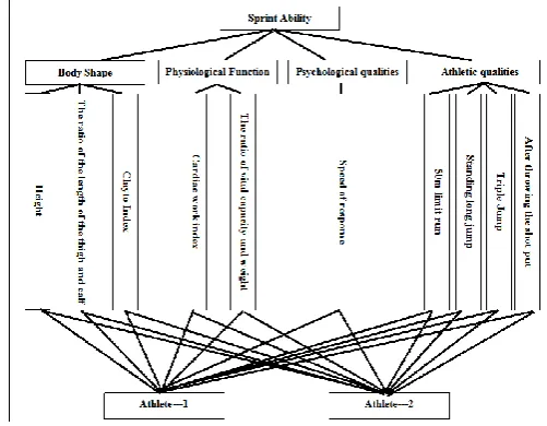
In Figure 1 step-1 indicates that the overall system is decomposed into a series of small parts. The sprint athletic capacity in this paper can be divided into physical shape, physiology, psychological quality and sports quality four major indicators; wherein body shape indicators include height, length ratio of thigh and calf and Quetlet index three small portions; physiological indicators include cardiac function index and vital capacity/weight values two small portions; the psychological quality indicators is mainly embodied by the sound reaction time; the sport quality indexes include 50m limit running, standing long jump, triple jump performance and back-throw shot distance four small parts, that is, the overall exercise capacity system is divided into four major terms and ten minor terms; Step-2 indicates that all the small parts after the system decomposition are assigned weights; Step-3 represents the assessment of all the small parts on the overall contribution ability to the athletic ability of athletes; Step-4 means that for the contribution ability of all the small parts on the athletic ability of different athletes obtain the evaluation results .
2.2 The hierarchical structure building of athletic ability
When research questions using the AHP method, according to the causal relationship of the various factors in the question it can be divided into several levels, called hierarchical. In this paper, the problem is relatively complex and is divided into four layers; the top layer is referred to as the goal layer and O layer for short that is athletic ability; the middle layer is the criterion layer and called C layer for short, it is divided into two layers respectively four major indicators C1 layer and its corresponding fraction content C2 layer; the bottom layer is the measures layer and called the P layer for short, that is two athletes. Figure 2 shows the hierarchical structure.
Figure 2: The hierarchical structure diagram of athletic ability
2.3 Assessment model building and algorithm design
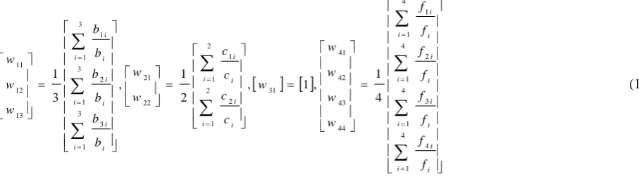
Definition 1: The weight representation between the first layer and the second layer is shown in the formula (1):
1
4 3 2
1 w w w
w (1)
[image:2.595.175.426.464.659.2]______________________________________________________________________________
weights of the body functions on athletic ability, w3means the contribution weights of the psychological quality on
athletic ability, and w4means the contribution weights of the athletic ability on athletic ability.
Definition 2: The weight representation between the second layer and the third layer is shown in the formula (2):
1 1 1 1
44 43 42 41
31 22 21
13 12 11
w w w w
w w w
w w w
(2)
In Formula (2), w11,w12,w13 respectively represents the contribution weights of height, leg length ratio and the
Quetlet index on the body shape; w21,w22 respectively represents the contribution weights of cardiac function
index and vital capacity/weight values on the physical function; w31 represents the contribution weights of sound
reaction time on the psychological quality, which is clearly one;w41,w42,w43,w44 respectively represents the contribution weights of 50m limit Race, standing long jump, triple jump performance and back-throw shot distance on the sport quality.
Definition 3: The weight representation between the third layer and the forth layer is shown in the formula (3):
1
2 1 ij
ij w
w (3)
In Formula (3) the meaning of wijk
[image:3.595.105.506.419.645.2]is shown in Table 1:
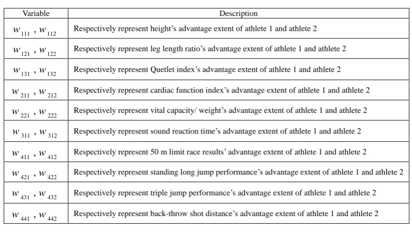
Table 1: Variable weights description
Variable Description
112 111 ,w
w Respectively represent height’s advantage extent of athlete 1 and athlete 2
122 121 ,w
w Respectively represent leg length ratio’s advantage extent of athlete 1 and athlete 2
132 131 ,w
w Respectively represent Quetlet index’s advantage extent of athlete 1 and athlete 2
212 211,w
w Respectively represent cardiac function index’s advantage extent of athlete 1 and athlete 2
222 221,w
w Respectively represent vital capacity/ weight’s advantage extent of athlete 1 and athlete 2
312 311 ,w
w Respectively represent sound reaction time’s advantage extent of athlete 1 and athlete 2
412 411,w
w Respectively represent 50 m limit race results’ advantage extent of athlete 1 and athlete 2
422 421,w
w Respectively represent standing long jump performance’s advantage extent of athlete 1 and athlete 2
432 431,w
w Respectively represent triple jump performance’s advantage extent of athlete 1 and athlete 2
442 441,w
w Respectively represent back-throw shot distance’s advantage extent of athlete 1 and athlete 2
Evaluation algorithm design:
Step-1: Calculation of the athletic ability index for athlete 1 is in the formula (4) below:
1 4
1
4 1 4 4
311 3 2
1
2 1 2 2
3
1
1 1 1
1 w w w w w w w w w w A
w
j
j j
j
j j
j
j
j
(4)
In Formula (4) A1means the athletic ability index of athlete 1.
2 4
1
4 2 4 4
312 3 2
1
2 2 2 2
3
1
1 2 1
1 w w w w w w w w w w A
w
j
j j j
j j j
j
j
(5)
In Formula (5) A2means the athletic ability index of athlete 2.
Step-3: Output the judgment result
WhenA1 A2, output "athlete 1's athletic ability is higher than athlete 2", whenA1 A2, output "athlete 2's athletic ability is higher than athlete 1."
2.4 The establishment of judgment matrix and weight generation algorithm design of each level
If you compare the impact size of n factors on certain factorF , we usually take the pair-wise factor comparison
method to establish judgment matrix. Supposeaij
indicates the influence ratio size of factori and factor j
on factorF , we can obtain the judgment matrixR ; In this paper we suppose the judgment matrix between the first
level and the second level isR1, the element isaij, the factor isi, j, the element isF1, then we have the
judgment matrixR1 as shown in the formula (6):
44 43 42 41 4
34 33 32 31 3
24 23 22 21 2
14 13 12 11 1
4 3 2 1 1
1
a a a a
a a a a
a a a a
a a a a F
R
(6)
In Formula (6), F1means factor athletic ability, 1,2,3,4means the body shape factor, physical function
factor, psychological factor and sport quality factor, aij
means the influence size of factori and factor j
on
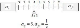
[image:4.595.225.393.467.526.2]factorF1. For the determination ofaij we usually use the 1~9 scale to assign the impact degree, as shown in Figure 3:
Figure 3: The assignment schematic of nine scale impact degree
Nine scale values are given in Table 2 below.
Table 2: Nine-scale schematic
Scale Meaning
1 The two elements have the same importance
3 The former element is slightly important than the latter element 5 The former element is obviously important than the latter element 7 The former element is strongly important than the latter element 9 The former element is extremely important than the latter element
The judgment matrixR2,R3,R4,R5 of the four groups of two-factori ~ j,i ~ j,i ~ j,i ~ j
for
factor F2,F3,F4,F5can be obtained, wherein the element is represented bybij,cij,dij, fij
______________________________________________________________________________
33 32 31 3 23 22 21 2 13 12 11 1 3 2 1 2 2 b b b b b b b b b F R (7) 22 21 2 12 11 1 2 1 3 3 c c c c F R (8) 11 1 1 4 4 d F R (9) 44 43 42 41 4 34 33 32 31 3 24 23 22 21 2 14 13 12 11 1 4 3 2 1 5 5 f f f f f f f f f f f f f f f f F R (10)TakingR1 for example, design the weight generation algorithm of each factor in the first level and the second level. Step-1: Calculate the additive sum for each column, as shown in the formula (11) below:
4 1 4 4 4 1 3 3 4 1 2 2 4 1 11 , , ,
i i i i i i i
i a a a a a a
a
a (11)
Step-2: All elements in each column are divided by the sum of the column and generate the matrixB1 as shown in formula (12) below:
4 44 3 43 2 42 1 41 4 34 3 33 2 32 1 31 4 24 3 23 2 22 1 21 4 14 3 13 2 12 1 11 1 a a a a a a a a a a a a a a a a a a a a a a a a a a a a a a a a
B (12)
Step-3: Calculating the average value of each row of the matrixB1, the average value is the weight between the second layer and the first layer as shown in formula (13):
4 1 4 4 1 3 4 1 2 4 1 1 44 43 42 41 31 2 1 2 2 1 1 22 21 3 1 3 3 1 2 3 1 1 13 12 11 4 1 , 1 , 2 1 , 3 1 i i i i i i i i i i i i i i i i i i i i i i i i i i i f f f f f f f f w w w w w c c c c w w b b b b b b w w w (14)2.5 Consistency checking algorithm design
As the complexity of the objective things are determined by the diversity of human, so in the constructing process of
the judgment matrixai j aj k ai k
does not have a strict set up; so in the calculation of the weight vector under a
single criterion, we must conduct consistency test. Carry through algorithm design taking matrixR1 for example, as follows:
Step-1: Obtain vectora
a1,a2,a3,a4
and vectorw
w1,w2,w3,w4
;
Step-2: Obtain the largest eigenvalue m ax of matrixR1, which is calculated as formula (15) below:
4 3 2 1 4 3 2 1 m ax w w w w a a a a w a (15)
Step-3: Calculate the consistency indexCI as calculated in formula (16) below:
3 4
3 1
m ax m ax
n n
CI (16)
In Formula (16) n represents the number of criteria, that is the number of factors, so for the matrixR1 n 4.
Step-4: Compute consistency ratio CR as calculated in formula (17):
RI CI
CR (17)
[image:6.595.75.529.78.207.2]In Formula (17) RI represents the Random Consistency Index value, as shown in Table 3.
Table 3: Consistency data
n 1 2 3 4 5 6 7 8 9 10
RI 0 0 0.58 0.9 1.12 1.24 1.32 1.41 1.45 1.49
Therefore, formula (17) can be rewritten as
9 . 0 3 4 max CR .
Step-5: Consistency judgments
______________________________________________________________________________
RESULTS
[image:7.595.157.453.133.349.2]3.1 The determination table of the relative weight for sprinter
Table 4: The compared weights of two sprinters and the corresponding index
Contrast value of indicators Variable Athlete 1 Athlete 2 Height
112 111 ,w
w 0.5437 0.4563
The ratio of the length of the thigh and calf
122 121 ,w
w 0.9608 0.0392
Quetlet Index
132 131 ,w
w 0.1744 0.8256
Cardiac work index
212 211,w
w 0.1571 0.8429
The ratio of vital capacity and weight
222 221,w
w 0.2681 0.7319
Speed of response
312 311 ,w
w 0.1775 0.8225
50m limit run
412 411,w
w 0.5768 0.4232
Standing long jump
422 421,w
w 0.4982 0.5018
Triple Jump
432 431,w
w 0.2852 0.7148
After throwing the shot put
442 441,w
w 0.1559 0.8441
3.2 Actual data filling of the judgment matrix
By pair-wise comparison between indicators judgment matrix Ri(i 1,2,3,4,5)can be obtained as in formula (18)
(19) (20) (21) and (22).
1 3 3 5
3 1 1 1 3
3 1 1 1 3
5 1
3 1
3 1 1
4 3 2 1
4 3 2 1 1
1
F
R (18)
1 3 7
3 1 1 5
7 1
5 1 1
3 2 1
3 2 1 2
2
F
R (19)
1 3
3 1 1
2 1
2 1 3
3
F
R (20)
1
1 1 4 4
F
1 5 1 3 1 9 1 5 1 3 5 1 3 3 1 1 7 1 9 5 7 1 4 3 2 1 4 3 2 1 5 5 F R (22)
3.3 Weight solving by Matlab
[image:8.595.66.524.47.693.2]According to the former algorithm use Matlab software programming, the program code is shown in Figure 4:
Figure 4: Weights solving and program code
The computational results are shown in Figure 5:
Figure 5: the results of weight solving by Matlab
Substituting the result into formula (13) and (14) then the formula (23) and (24) can be obtained.
5222 . 0 1998 . 1 1998 . 0 0781 . 0 4 3 2 1 w w w w (23)
0457 . 0 2027 . 0 0942 . 0 6574 . 0 , 1 , 7500 . 0 2500 . 0 , 6491 . 0 2790 . 0 0719 . 0 44 43 42 41 31 22 21 13 12 11 w w w w w w w w w w (24)3.5 Consistency test achieved Matlab
______________________________________________________________________________
Figure 6: the consistency test of judgment matrix achieved by Matlab
Test results are shown in Figure 7:
Figure 7: Consistency test results
From the consistency judgment results in Figure 7 the judgment matrix built in this paper shows considerable consistency.
Based on the above obtained data and evaluation algorithm in 2.3, , by using Matlab symbolic computation we can
get the athletic ability indexA1 0.37274451 203, A2 0.627155488 of athlete 1 and athletes 2, obviouslyA2 A1, that is athlete 2's athletic ability is higher than athlete 1.
CONCLUSION
AHP well evaluates sprint athletic ability, and has been demonstrated with actual data; This paper builds a significant consistency of judgment matrix; the selected indicators also reflect a sprinter's athletic ability; The algorithms described in this article is concise, which not only can be implemented in Matlab, but also can be achieved by other software, such as C + +, VB, etc. This article evaluates two athletes, while simultaneously evaluating several athletes’ athletic ability it can achieve well two. This paper describes sprinter’s athletic ability by the use of AHP, meanwhile designs the weight algorithms of the judgment matrix and algorithms of the overall consistency checking, programs based on the algorithm, uses Matlab software to achieve the AHP analysis of the actual parameters for the two athletes, obtains the pros and cons of two athletes’ athletic ability, and passes the consistency test.
REFERENCES
[1]Bing Zhang,Hui Yue, 2013, International Journal of Applied Mathematics and Statistics, 40(14), 469-476. [2]Deng Yunling, Zhang Guanglin & Xu Shiyan,2007, Northwest Normal University Journal: Natural Science
[3]Du Heping,2006, Guangzhou Physical Education Institute Jounal, 26(5),85-87.
[4]Haibin Wang, Shuye Yang, 2013, International Journal of Applied Mathematics and Statistics, 39(9), 243-250. [5]He Hua, Li Yanpeng,2008, Hubei Sports Science and Technology, 27(1),50-52.
[6]Peng Haifeng,Duan Yuxiang & Ding Hairong, Wu Xudong,2007, China Sports Coaches, (2),52-53. [7]Wang Peng,2009, Sports Science Research, (1), 65-67.
[8]Ye Shengshun,2005, Jilin Institute of Physical Education Journal, 21(4),62-63.