Determination of Wireless Communication Links
Optimal Transmission Range Using Improved
Bisection Algorithm
Enyenihi Henry Johnson1, Simeon Ozuomba2,*, Ifiok Okon Asuquo2
1Department of Electrical/Electronic Engineering, Akwa Ibom State University, Nigeria 2Department of Electrical/Electronic and Computer Engineering, University of Uyo, Nigeria
Copyright©2019 by authors, all rights reserved. Authors agree that this article remains permanently open access under the terms of the Creative Commons Attribution License 4.0 International License
Abstract In this paper, an improved bisection
algorithm for computing the optimal transmission range of wireless communication links was presented. The optimal path length is based on the link budget equation for line-of-sight wireless communication links. Specifically, free space path loss model was used for the clear-air path loss while multipath fading and rain fading were the two fade mechanisms considered in the determination of the expected fade margin. Sample numerical example was carried out for a frequency of 10 GHz and a site located in the International Telecommunication Union (ITU) rain zone N. The result showed that at 10 GHz and with the given network and link parameters, the improved bisection algorithm converged at the 7th cycle while the classical bisection method converged at the 12th cycle. Further numerical examples were examined for frequencies ranging from 10 GHz to 200 GHz. In all, the improved bisection method had at least 41 % reduction in the convergence cycle when compared with that of the classical bisection method. A similar study with the classical Newton-Raphson method converged at the 4th cycle for a 12 GHz signal while the improved bisection method converged at the 6th cycle. Essentially, the Newton-Raphson method converges faster than the bisection and the improved bisection methods. However, it is very difficult to apply the classical Newton-Raphson method when several clear-air path losses are to be considered or when complex path loss model such as the Hata model is used in the path loss computation. As such, the improved bisection method is preferred due to its simplicity and also it offers convergence performance that is comparable to that of the classical Newton-Raphson method.Keywords
Bisection Method, Adjustment Value for Iteration Variable, Line-of-sight Links, Rain Fade Depth, Multipath Fade Depth1. Introduction
Today, there are several numerical iteration methods for solving non-linear equations [1, 2, 3, 4, 5]. Among the numerical iteration methods, the Newton-Raphson method and the bisection method are the most popular [6, 7, 8, 9]. However, the two methods in their original forms have been associated with some shortcomings. The classical Newton-Raphson method requires some extra mathematical processes that make it difficult to be applied in many cases [10, 11, 12, 13]. On the other hand, the classical bisection method is quite simple; however, when compared to the other methods, the bisection method takes longer time to converge [14, 15, 16, 17, 18]. Consequently, variants of the classical Newton-Raphson method and bisection method have been developed.
convergence performance than the classical bisection method.
Notably, in the line-of-sight (LOS) wireless communication links, the maximum transmission range is always required to determine the maximum distance between the transmitter and the receiver. At the maximum transmission range, it is expected that the network will still meet the performance requirements [20, 21, 22, 23, 24, 25, 26]. However, a recent study proposed optimal transmission range at which point the available fade margin in the link can accommodate the maximum fade depth that can occur in the link based on the design specifications. Although such optimal length computation has been done using the classical Newton-Raphson method [27], in this paper, the modified bisection method is presented due to its simplicity and comparable convergence performance with the Newton-Raphson method.
The study is carried out in Imo state, Nigeria where multipath fading and rain fading are the two major fade mechanisms mostly considered in wireless network design. Furthermore, mutual exclusive relationship exists among multipath fading, and rain fading [28]. As such, in practice, the fade mechanism with higher fade depth is considered as the effective fade mechanism for the communication link. In addition, in locations where only multipath and rain fade mechanisms are considered, for frequencies above 10 GHz, rain fading dominates whereas; the multipath fading dominates at the lower frequencies [29,30,31]. In addition, according to [27], when multipath fading dominates, the optimal path length can be determined using a close-form solution. However, when rain fading dominates, the resulting mathematical expression leads to a product log function that does not have a closed-form solution. As such, a numerical method or the Lambert W function approach can be used to determine the optimal path length [27]. In this paper, a modified bisection numerical method is used. The study focused on the frequencies above 10 GHz where the rain fading is the dominant fade mechanism for the case study area.
In all, the main motive for the study is to derive a simple numerical iteration method that can be used to determine the optimal path length in the tropical regions where rain fading and multipath fading are the prevailing fade mechanisms. Presently, available studies on the optimal path length focused on free space path loss as the only loss the signal will experience along with the rain or multipath fading. However, there are other complex path loss models and also additional path losses due to diffraction effect of obstructions in the signal path. When such complex path losses models and diffraction path loss are considered, it will become extremely difficult to use the classical Newton-Raphson method. As such, a simpler numerical iteration method, like the improved bisection method is needed since it can also give good convergence performance comparable to that of the classical Newton-Raphson method.
2. Determination of Maximum
Transmission Range for
Line-of-sight (Los) Wireless
Communication Links
The received signal strength, PR of LOS link is given as
follows [20]:
PR = 𝑓𝑓𝑓𝑓𝑠𝑠 + 𝑃𝑃𝑆 = PT + (GT + GR ) – LFSP (1)
Where;
fms = fade margin (dBm) Ps = receiver sensitivity (dBm) PR = Received Signal Power (dBm)
PT = Transmitter Power Output (dBm)
GT = Transmitter Antenna Gain (dBi)
GR = Receiver Antenna Gain (dBi)
LFSP = Free Space Path Loss (dB).
If the frequency, f is in GHz and d is given in km, then, LFSP is given as;
LFSP = 32.4 + 20 log (f*1000) + 20 log (d) (2) The transmission range (d) can be determined from Equations 1 to 2 as follows:
d = 10��PT + GT+GR−𝑓𝑚𝑠−𝑃𝑆20�−32.4−20log(f∗1000) � (3)
The fade depth Amultipath (dB) can be determined from
the ITU multipath fading model for quick planning applications which is expressed as [27];
𝑝𝑜 = Kd3.1(1+|ε
P|)-1.29 (𝑓𝑓0.8) 10
�−0.00089ℎ𝐿𝐿− �𝑨𝑚𝑢𝑢𝑙𝑡𝑖𝑢𝑢𝑎𝑡ℎ�𝟏𝟏𝟎 �
(4) Where:
𝑃𝑃𝑜 is the percentage of time that 𝑨𝑓𝑓𝑢𝑢𝑙𝑙𝑡𝑖𝑢𝑢𝑎𝑡ℎ is
exceeded in the average worst month
d is the propagation transmission range or distance (in km) between the transmitter and the receiver
f is frequency (GHz)
hL is altitude of lower antenna (m)
Amultipath is multipath fade depth (dB)
𝑓𝑓𝑁1 is point refractivity gradient
K is geoklimatic factor and can be obtained from:
K = 10(−4.6−0.0027𝑑𝑁1) (5)
εP is the path inclination, (in mrad). εP is calculated using
the following expression
�𝜺𝒑�= (|𝒉𝒕−𝒉𝒇𝒇 𝒓|) (6)
where:
d is the propagation transmission range or distance (in km) between the transmitter and the receiver
ℎ𝑡 is the antenna transmitter antenna height
ℎ𝑟 is the receiver transmitter antenna height (where ℎ𝑡
ℎ𝐿𝐿 =𝑓𝑓𝑖𝑛𝑖𝑓𝑓𝑢𝑓𝑓(ℎ𝑡,ℎ𝑟) (7)
Hence, the multipath fade depth, 𝑨𝑓𝑓𝑢𝑢𝑙𝑙𝑡𝑖𝑢𝑢𝑎𝑡ℎ (in dB) is obtained from the expression for 𝑃𝑃𝑜 as follows;
𝑨𝑓𝑓𝑢𝑢𝑙𝑙𝑡𝑖𝑢𝑢𝑎𝑡ℎ= 10(−0.00089ℎ𝐿𝐿)−(10)log��𝐾(𝑑3.1)�1+�𝜀𝑢𝑢𝑜𝑜
𝑢𝑢��−1.29(𝑓𝑓0.8)�� (8)
The ITU-R PN.838 recommendations specified the specific attenuation originating from rainfall as γRpo in dB/km and
modeled it using the power-law relationship as follows [27] ;
𝛾𝑅𝑢𝑢𝑜= 𝑘�𝑅𝑢𝑢𝑜𝑜�
𝛼
(9) Where 𝑅𝑢𝑢𝑜𝑜 is the rainfall rate in mm/h exceeded for 𝑃𝑃𝑜% of an average year (or stated another way, 𝑅𝑢𝑢𝑜𝑜 is the rainfall rate in mm/h for a particular link percentage outage, Po). k and α are frequency dependent. The rain fade depth,
𝐴𝑅𝑎𝑖𝑛𝑛 for a transmission range, d (in Km) is given as
𝐴𝑅𝑎𝑖𝑛𝑛=�𝛾𝑅𝑢𝑢𝑜� 𝑓𝑓= �𝑘�𝑅𝑢𝑢𝑜𝑜�
𝛼
�𝑓𝑓 (10)
In reality, k and α are given for the vertical polarization and horizontal polarization and hence, 𝐴𝑅𝑎𝑖𝑛𝑛 is computed for
vertical polarization and horizontal polarization and the larger of the two is the effective rain fade depth.
In all, the larger of the rain fade depth and multipath fade depth is taken as the link maximum fade depth (𝑓𝑓𝑓𝑓𝑓𝑓) and it is
expressed as;
𝑓𝑓𝑓𝑓𝑓𝑓 = 𝑓𝑓𝑎𝑥𝑥𝑖𝑓𝑓𝑢𝑓𝑓�𝑨𝑓𝑓𝑢𝑢𝑙𝑙𝑡𝑖𝑢𝑢𝑎𝑡ℎ, 𝐴𝑅𝑎𝑖𝑛𝑛� (11)
The optimal transmission range (dmop) is obtained when the following condition is fulfilled;
𝑓𝑓𝑓𝑓𝑓𝑓= 𝑃𝑃𝑅−𝑃𝑃𝑆 (12)
3. Development of the Improved Bisection Algorithm for the Determination of
Optimal Transmission Range
3.1. Theory of the Improved Bisection Method for the Determination of Optimal Transmission Range
The bisection method is a binary search method that is used to find the root of an equation, such as function f(x) in a given interval, where the root is the value of ‘x’ for which f(x) = 0. The bisection method is based on the intermediate value theorem which states that if f(x) is a continuous function and there are two real numbers a and b such that f(a)*f(b) 0 and f(b) < 0), then it is guaranteed that it has at least one root between them. Given that X𝑢𝑢𝑢𝑢=𝑏, X𝐿𝐿𝑛𝑛=𝑎 and
X𝑛𝑛𝑛𝑛𝑛𝑛=𝑐 the bisection method can be stated as follows;
X𝑛𝑛𝑛𝑛𝑛𝑛 = �X𝑢𝑢𝑢𝑢−X2 𝐿𝐿𝐿𝐿� (13)
X𝑛𝑛𝑛𝑛𝑛𝑛= �X𝑢𝑢𝑢𝑢−X𝛽 𝐿𝐿𝐿𝐿� (14)
Steps for performing the bisection method are as follows: 1. Set or initialize the error tolerance, 𝜖𝜖𝑠𝑠
2. Find middle point X𝑛𝑛𝑛𝑛𝑛𝑛= �X𝑢𝑢𝑢𝑢−X2 𝐿𝐿𝐿𝐿�
3. If f (X𝑛𝑛𝑛𝑛𝑛𝑛) = 0 or f (X𝑛𝑛𝑛𝑛𝑛𝑛) < 𝜖𝜖𝑠𝑠 then Stop // X𝑛𝑛𝑛𝑛𝑛𝑛 is the root of the solution.
4. Else If value f(X𝐿𝐿𝑛𝑛)*f(X𝑛𝑛𝑛𝑛𝑛𝑛)) < 0 then
X𝑢𝑢𝑢𝑢 = X𝑛𝑛𝑛𝑛𝑛𝑛 // root lies between X𝐿𝐿𝑛𝑛 and X𝑛𝑛𝑛𝑛𝑛𝑛.go to step 1 // recur for X𝐿𝐿𝑛𝑛 and X𝑛𝑛𝑛𝑛𝑛𝑛
5. Else If f(X𝑢𝑢𝑢𝑢)*f(X𝑛𝑛𝑛𝑛𝑛𝑛) < 0 then
X𝐿𝐿𝑛𝑛 = X𝑛𝑛𝑛𝑛𝑛𝑛 // root lies between X𝑛𝑛𝑛𝑛𝑛𝑛 and X𝑢𝑢𝑢𝑢 go to step 1 // recur for X𝑛𝑛𝑛𝑛𝑛𝑛 and X𝑢𝑢𝑢𝑢
6. Else Stop // given function does not follow one of the assumptions.
3.2. The Improved Bisection Algorithm for the Determination of the Optimal Transmission Range of Line-of-sight Wireless Communication Links
X𝑛𝑛𝑛𝑛𝑛𝑛= �X𝑢𝑢𝑢𝑢−𝛽X𝐿𝐿𝑛𝑛�
For the classic bisection method 𝛽= 2, hence
X𝑛𝑛𝑛𝑛𝑛𝑛 = �X𝑢𝑢𝑢𝑢−𝛽X𝐿𝐿𝑛𝑛� = X𝑢𝑢𝑢𝑢−2X𝐿𝐿𝑛𝑛
Although, bisection method uses 𝛽= 2 with little knowledge of the prevailing link parameters, the 𝛽 factor can be improved to suit the link operating conditions. In this research, 𝛽 is defined as;
𝛽 =�X X𝑢𝑢𝑢𝑢 𝑢𝑢𝑢𝑢−X𝐿𝐿𝑛𝑛�
Consider a numerical example where X𝐿𝐿𝑛𝑛 =16 and X𝑢𝑢𝑢𝑢 =102 then
𝛽 =�X X𝑢𝑢𝑢𝑢
𝑢𝑢𝑢𝑢−X𝐿𝐿𝑛𝑛�=�
102
102−16 �= 1.186 Hence,
X𝑛𝑛𝑛𝑛𝑛𝑛= �X𝑢𝑢𝑢𝑢−𝛽X𝐿𝐿𝑛𝑛� = �1021.186−16�= 72.513
For the classical bisection method with 𝛽 =2 the value of X𝑛𝑛𝑛𝑛𝑛𝑛will be
X𝑛𝑛𝑛𝑛𝑛𝑛= �1022−16�= 1 43
As can be seen, whereas the bisection method will use 𝛽= 2, the improved bisection method will use 𝛽= 1.186. The adjusted value of 𝛽 is expected to give rise to faster convergence of the algorithm. As regards the optimal transmission range of the microwave links, the bisection method uses 𝛽= 2 because it has little knowledge of the prevailing link parameters. In this paper, given that the fade margin at design time specification is denoted as 𝑓𝑓𝑓𝑓𝑠𝑠 and the corresponding
fade depth is denoted as 𝑓𝑓𝑓𝑓𝑓𝑓, then; 𝑓𝑓𝑓𝑓𝑓𝑓=𝑓𝑓𝑓𝑓𝑠𝑠 and 𝛽=�𝑓𝑓𝑑𝑚𝑓𝑓𝑑−𝑓𝑓𝑓𝑓𝑛𝑛𝑚 � . Now consider a numerical example, if 𝑓𝑓𝑓𝑓𝑓𝑓= 𝑓𝑓𝑓𝑓𝑠𝑠=19.96 dB and 𝑓𝑓𝑓𝑓𝑓𝑓 =124.83 dB then;
𝛽=�𝑓𝑓𝑓𝑓 𝑓𝑓𝑓𝑓𝑓𝑓
𝑓𝑓− 𝑓𝑓𝑓𝑓𝑓𝑓�=�
124.83 124.83 −19.96�=
124.83
104.87 = 1.1903
As can be seen, whereas the bisection method will use𝛽= 2, the improved bisection method will use 𝛽= 1.1903. The improved 𝛽 value is expected to give rise to faster convergence of the algorithm. The algorithm for the improved bisection method is the same as the classical bisection method present in this chapter except that in the improved bisection method the value of 𝛽 must be computed first and used in the iteration.
𝛽=�𝑓𝑓𝑓𝑓 𝑓𝑓𝑓𝑓𝑓𝑓 𝑓𝑓− 𝑓𝑓𝑓𝑓𝑓𝑓�
The algorithm for the improved bisection method for optimal transmission range is given as follows; Step 1: Specify requisite link parameters values
Specify the following parameters (i) 𝑃𝑃𝑠𝑠 = the receiver sensitivity in dB
(ii) 𝑓𝑓𝑓𝑓𝑠𝑠 the specified (required) fade margin in dB
(iii) PT = the transmitter power output (dBm) (iv) GT = the transmitter antenna gain (dBi) (v) GR = the receiver antenna gain (dBi)
(vi) LT = the losses from transmitter (cable, connectors etc.) (dB) (vii)LR = the losses from receiver (cable, connectors etc.) (dB)
(viii)LM = the miscellaneous losses (fade margin, polarization misalignment etc.) (dB) (ix) Specified relative error tolerance, 𝜖𝜖𝑠𝑠 where 𝜖𝜖𝑠𝑠= 0.01% =0.01100 = 0.0001
Step 2: Initialize the parameters
Step 2.3 ∈𝑠𝑠 = 0.01%
Step 2.4 𝑗𝑗= 0 // j is iteration counter
Step 3 Compute the operating free space path loss, 𝐋𝐋𝐅𝐅𝐅𝐅𝐅𝐅 and set the initial operating free space path loss, 𝐋𝐋𝐅𝐅𝐅𝐅𝐅𝐅(𝐤𝐤)
Step 3.1
Compute 𝑃𝑃𝑅 , the received signal power in dB as follows;
𝑃𝑃𝑅 = 𝑓𝑓𝑓𝑓𝑓𝑓(𝑘𝑘) + 𝑃𝑃𝑆
Step 3.2
Compute LFSP, the Free Space Path Loss (dB) as follows;
LFSP = PT + GT + GR - PR = PT + GT + GR - 𝑓𝑓𝑓𝑓𝑓𝑓(𝑘𝑘)−𝑃𝑃𝑆
Step 3.3
Set the initial operating free space path loss, 𝐋𝐋𝐅𝐅𝐅𝐅𝐅𝐅(𝟎)
LFSPe(k)= LFSP
Step 3.4
Compute the operating fade depth, 𝒇𝒇𝒇𝒇𝒇𝒇 and set the initial effective operating fade margin, 𝑓𝑓𝑓𝑓𝑓𝑓𝑛𝑛(𝑘𝑘)
Step 3.5
Compute d, the length of the link in km as follows;
d = 10�
LFSP(k)−32.4−20log(f∗1000)
20 � =10�� PT + GT+GR −PR20 �−32.4−20log(f∗1000) �
Step 3.6
Compute 𝐴𝑅𝑎𝑖𝑛𝑛, the operating rain fade depth in dB as follows; 𝐴𝑅(ℎ) = �〈γRpo〉h�d =�Kh�Rpo�
αh�d
𝐴𝑅(𝑣) = �〈γRpo〉v�d =�Kv�Rpo�
αv�d �
𝐴𝑅𝑎𝑖𝑛𝑛 = max��Kv�Rpo�αv� ∗ �Kh�Rpo�αh� ∗d� = max�𝐴𝑅(ℎ),𝐴𝑅(𝑣)� d 𝐴𝑅𝑎𝑖𝑛𝑛(𝑗𝑗) =𝐴𝑅𝑎𝑖𝑛𝑛
Step 3.7
Compute the operating multipath fade depth, 𝑨𝑓𝑓𝑢𝑢𝑙𝑙𝑡𝑖𝑢𝑢𝑎𝑡ℎ in dB as follows;
𝑨𝑓𝑓𝑢𝑢𝑙𝑙𝑡𝑖𝑢𝑢𝑎𝑡ℎ= 10(−0.00089ℎ𝐿𝐿)−(10)log� 𝑝𝑜 �𝐾(𝑓𝑓3.1)�1 +�𝜀
𝑢𝑢��−1.29(𝑓𝑓0.8)� �
Step 3.8
Compute the operating fade depth, 𝑓𝑓𝑓𝑓𝑓𝑓 in dB as follows;
𝑓𝑓𝑓𝑓𝑓𝑓= max�𝑨𝑓𝑓𝑢𝑢𝑙𝑙𝑡𝑖𝑢𝑢𝑎𝑡ℎ, 𝐴𝑅𝑎𝑖𝑛𝑛�=𝑓𝑓𝑎𝑥𝑥 �𝑨𝑓𝑓𝑢𝑢𝑙𝑙𝑡𝑖𝑢𝑢𝑎𝑡ℎ,�max�𝐴𝑅(ℎ),𝐴𝑅(𝑣)���
Step 3.9
Set the initial effective operating fade margin, 𝑓𝑓𝑓𝑓𝑓𝑓𝑛𝑛(𝑘𝑘)
𝑓𝑓𝑓𝑓𝑓𝑓𝑛𝑛(𝑘𝑘)=𝑓𝑓𝑓𝑓𝑓𝑓
Step 4
K = K+ 1: Increase k by 1
Step 5 Use the values of 𝒇𝒇𝒇𝒇𝒇𝒇(𝒌𝒌−𝟏𝟏) and 𝒇𝒇𝒇𝒇𝒇𝒇𝒇𝒇(𝒌𝒌−𝟏𝟏) to determine the adjustment value where the adjustment value
is denoted as 𝜟𝜟𝒇𝒇𝒇𝒇𝒇𝒇(𝒌𝒌)
Step 5.1 Set the two values 𝑥𝑥𝑙𝑙(𝑘𝑘) and 𝑥𝑥𝑢𝑢(𝑘𝑘) for fade margin where;
𝑥𝑥𝑢𝑢(𝑘𝑘) =𝑓𝑓𝑎𝑥𝑥𝑖𝑓𝑓𝑢𝑓𝑓�𝑓𝑓𝑓𝑓𝑓𝑓(𝑘𝑘−1),𝑓𝑓𝑓𝑓𝑓𝑓𝑛𝑛(𝑘𝑘−1)�
Step 5.2 Determine the adjustment value for 𝑓𝑓𝑓𝑓(𝑘𝑘−1)
where the adjustment value, 𝛥𝛥𝑓𝑓𝑓𝑓 is the a point between 𝑥𝑥𝑙𝑙(𝑘𝑘) and 𝑥𝑥𝑢𝑢(𝑘𝑘) obtain as follows;
𝛽 =�𝑥𝑥 𝑥𝑥𝑢𝑢(𝑘𝑘) 𝑢𝑢(𝑘𝑘)− 𝑥𝑥𝑙𝑙(𝑘𝑘)�
𝛥𝛥𝑓𝑓𝑓𝑓=𝑥𝑥𝑓𝑓(𝑘𝑘)=𝑥𝑥𝑢𝑢(𝑘𝑘)−𝛽 𝑥𝑥𝑙𝑙(𝑘𝑘)
𝛥𝛥𝑓𝑓𝑓𝑓(𝑗𝑗)=𝛥𝛥𝑓𝑓𝑓𝑓
Step 6 Determine the adjusted value for 𝒇𝒇𝒇𝒇𝒇𝒇𝒇𝒇(𝒌𝒌) where
the adjustment value, 𝒇𝒇𝒇𝒇𝒇𝒇𝒇𝒇(𝒌𝒌) is given as; 𝑓𝑓𝑓𝑓𝑓𝑓𝑛𝑛(𝑘𝑘) =𝑓𝑓𝑓𝑓𝑓𝑓𝑛𝑛(𝑘𝑘−1)+ 𝛥𝛥𝑓𝑓𝑓𝑓 if 𝑥𝑥𝑙𝑙(𝑘𝑘)=𝑓𝑓𝑓𝑓𝑓𝑓𝑛𝑛(𝑘𝑘−1) 𝑓𝑓𝑓𝑓𝑓𝑓𝑛𝑛(𝑘𝑘) =𝑓𝑓𝑓𝑓𝑓𝑓𝑛𝑛(𝑘𝑘−1)− 𝛥𝛥𝑓𝑓𝑓𝑓 if 𝑥𝑥𝑢𝑢(𝑘𝑘)= 𝑓𝑓𝑓𝑓𝑓𝑓𝑛𝑛(𝑘𝑘−1)
Step 7
Determine the adjusted value for optimal transmission range, 𝑓𝑓𝑛𝑛(𝑘𝑘) where the adjusted value is given as;
If �𝐴𝑛𝑛𝑅(ℎ) ≥ 𝐴𝑛𝑛𝑅(𝑣)� then �γRpo=〈γRpo〉h�
otherwise �γRpo =〈γRpo〉v�. Then
𝑓𝑓𝑛𝑛(𝑘𝑘) = 𝑓𝑓𝑓𝑓𝛾𝑓𝑓𝑛𝑛(𝑘𝑘) 𝑅𝑢𝑢𝑜
Step 8
Determine the adjusted value for effective free space path loss, LFSPe(k) where the adjustment value is given as;
LFSPe(k) = 32.4 + 20 log(f*1000) + 20 log(𝑓𝑓𝑛𝑛(𝑘𝑘))
Step 9
Determine the adjusted value for effective fade margin where the adjusted value is given from as;
𝑓𝑓𝑓𝑓𝑛𝑛(k) = (LFSP +𝑓𝑓𝑓𝑓𝑠𝑠)−LFSPe(k)
Step 10
Check if the optimal transmission range condition is met, that is if;
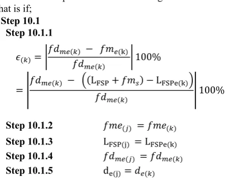
Step 10.1 Step 10.1.1
𝜖𝜖(𝑘𝑘)=�𝑓𝑓𝑓𝑓𝑓𝑓𝑛𝑛(𝑘𝑘)𝑓𝑓𝑓𝑓− 𝑓𝑓𝑓𝑓𝑛𝑛(k) 𝑓𝑓𝑛𝑛(𝑘𝑘) �100%
=�𝑓𝑓𝑓𝑓𝑓𝑓𝑛𝑛(𝑘𝑘) − �(L𝑓𝑓𝑓𝑓FSP+𝑓𝑓𝑓𝑓𝑠𝑠)−LFSPe(k)�
𝑓𝑓𝑛𝑛(𝑘𝑘) �100%
Step 10.1.2 𝑓𝑓𝑓𝑓𝑓𝑓(𝑗𝑗) =𝑓𝑓𝑓𝑓𝑓𝑓(𝑘𝑘)
Step 10.1.3 LFSP(j) = LFSPe(k)
Step 10.1.4 𝑓𝑓𝑓𝑓𝑓𝑓𝑛𝑛(𝑗𝑗) =𝑓𝑓𝑓𝑓𝑓𝑓𝑛𝑛(𝑘𝑘)
Step 10.1.5 de(j)=𝑓𝑓𝑛𝑛(𝑘𝑘)
Step 10.1.6 𝜖𝜖(𝑗𝑗)=𝜖𝜖(𝑘𝑘)
Step 10.2
If �𝜖𝜖(𝑘𝑘)% > |∈𝒔𝒔 %|� Then
Goto Step 4 Else
Goto Step 11 Endif
Step 11
Step 11.1 𝑓𝑓𝑓𝑓𝑓𝑓𝑜𝑜𝑢𝑢 =𝑓𝑓𝑓𝑓𝑓𝑓(𝑘𝑘)
Step 11.2 LFSPop = LFSPe(k)
Step 11.3 𝑓𝑓𝑓𝑓𝑓𝑓𝑜𝑜𝑢𝑢 =𝑓𝑓𝑓𝑓𝑓𝑓𝑛𝑛(𝑘𝑘)
Step 11.4 dmop=𝑓𝑓𝑛𝑛(𝑘𝑘)
Step 11.5 𝜖𝜖𝑜𝑜𝑢𝑢(𝑗𝑗)=𝜖𝜖(𝑘𝑘)
Step 12 Stop
4. Results and Discussions
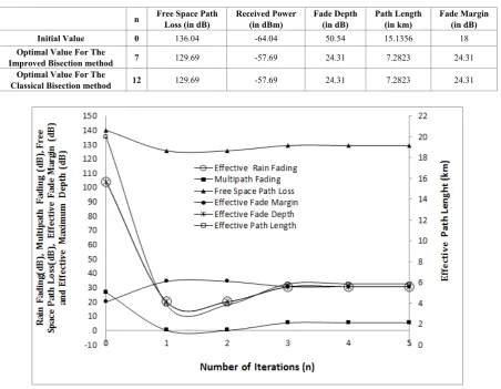
[image:6.595.61.289.579.754.2]In the sample numerical computation which the results are shown in Table 1 and Table 2, as well as Figure 1 and Figure 2, the frequency is 10 GHz, the transmitter power is 12 dB, the transmitter antenna gain is 30 dBi, the receiver antenna gain is 30 dBi, the receiver sensitivity is -82 dB, the fade margin is 18 dB, the network percentage availability is 99.99%, the ITU rain zone is N and hence the rain rate is 95 mm.hr, the rain fading constants are; 𝑘h =
0.01217, 𝑎h = 1.2571, 𝑘v =0.01129 and 𝑎v = 1.2156.
The convergence cycle for the improved bisection method is 7. That means, as shown in Table 1 and Table 2 (as well as, Figure 1 and Figure 2), the improved bisection algorithm is iterated for 7 times before the optimal transmission range is obtained. Also, the optimal transmission range is 7.28226 km, the optimal free space path loss is 129.69 dB, the optimal fade margin the system can accommodate is 24.31 dB and the optimal fade depth value is 24.31 dB. In essence, for the improved bisection algorithm, at the optimal transmission range, a maximum fade depth of 24.31dB can be accommodated by the link which is the same with the optimal fade depth value of 24.31 dB. It can be seen from Table 2 and Figure 2 that the initial fade margin specified for the system is 18 dB. At this initial point, in Table 2 and Figure 2, the initial maximum transmission range is 15.1356 km, the initial path loss is 136.04 dB, and the initial fade depth is 50.54 dB while the initial received signal power is -60.04 dB. At the optimal point, the path maximum path loss has reduced by 6.35 dB to a value of 129.69 dB while the received signal power has increased the same value of -60.04 dB to a value of -57.69 dB From Table 1 and Figure 1, it will be noticed that the rain fading is equal to the effective fade depth. In essence, for the given frequency, rain zone and percentage availability, the rain fading is greater than the multipath fading and hence, determines the effective fade depth that will be experienced in the link.
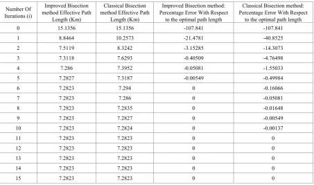
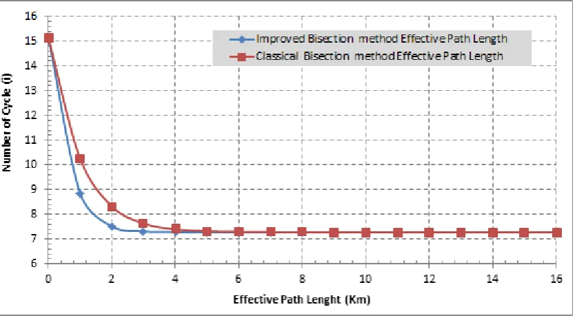
as well as the percentage error with respect to the optimal path length for the improved bisection method and the classical bisection method is shown in Table 3 and Figure 3. The two models started with initial percentage error of -107.841 5 but at the end of the first iteration (i=1) the improve bisection method recorded percentage error of
-21.4781 % whereas the classical bisection method recorded -40.8525 %. In all, the improved bisection method converges faster than the classical bisection method. Consequently, the improved bisection method converged at the 7th cycle (i=7) whereas the classical
[image:7.595.68.530.183.293.2]bisection method converged at the 12th cycle.
Table 1. Improved bisection method: how the key link parameters vary with number of iterations (n)
Number Of
Iterations (n) Effective Rain Fading Free Space Path Loss Multipath Fading Effective Path Length Effective Fade Depth Effective Fade Margin
0 50.54 136.04 21.29 15.13561 50.54 17.96
1 29.54 131.38 12.01 8.84641 29.54 22.62
2 25.08 129.95 9.11 7.51187 25.08 24.05
3 24.41 129.72 8.63 7.31180 24.41 24.28
4 24.33 129.69 8.57 7.28597 24.33 24.31
[image:7.595.75.528.326.677.2]5 24.32 129.69 8.56 7.28273 24.32 24.31
Table 2. Improved bisection method and the classical bisection method: initial free space path loss, optimal values for free space path loss, fade depth, fade margin, path length and convergence cycle
n Free Space Path Loss (in dB) Received Power (in dBm) Fade Depth (in dB) Path Length (in km) Fade Margin (in dB)
Initial Value 0 136.04 -64.04 50.54 15.1356 18
Optimal Value For The
Improved Bisection method 7 129.69 -57.69 24.31 7.2823 24.31 Optimal Value For The
Classical Bisection method 12 129.69 -57.69 24.31 7.2823 24.31
Figure 2. Improved bisection method and the classical bisection method: initial free space path loss, optimal values for free space path loss, fade depth, fade margin, path length and convergence cycle
Table 3. Improved bisection method and the classical bisection method: effective path length versus number of iterations (n)
Number Of Iterations (i)
Improved Bisection method Effective Path
Length (Km)
Classical Bisection method Effective Path
Length (Km)
Improved Bisection method: Percentage Error With Respect
to the optimal path length
Classical Bisection method: Percentage Error With Respect
to the optimal path length
0 15.1356 15.1356 -107.841 -107.841
1 8.8464 10.2573 -21.4781 -40.8525
2 7.5119 8.3242 -3.15285 -14.3073
3 7.3118 7.6293 -0.40509 -4.76498
4 7.286 7.3952 -0.05081 -1.55033
5 7.2827 7.3187 -0.00549 -0.49984
6 7.2823 7.294 0 -0.16066
7 7.2823 7.286 0 -0.05081
8 7.2823 7.2835 0 -0.01648
9 7.2823 7.2827 0 -0.00549
10 7.2823 7.2824 0 -0.00137
11 7.2823 7.2823 0 0
12 7.2823 7.2823 0 0
13 7.2823 7.2823 0 0
14 7.2823 7.2823 0 0
[image:8.595.72.526.331.598.2]Figure 3. Improved bisection method and the classical bisection method: effective path length versus number of iterations (n)
Table 4. Improved bisection method: effect of frequency on optimal path length, initial path length and convergence cycle
f (GHz) Convergence Cycle Initial Path Length (km) Optimal Path Length (km)
10 7 15.14 7.28
20 5 7.57 2.47
30 5 5.05 1.48
40 5 3.78 1.13
50 5 3.03 0.97
60 4 2.52 0.89
70 5 2.16 0.83
80 5 1.89 0.79
90 6 1.68 0.76
100 7 1.51 0.74
150 8 1.01 0.08
200 8 0.76 0.05
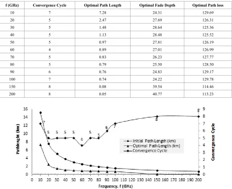
Effect of Frequency: Table 4, Table 5 and Table 6 (as well as, Figure 4 to Figure 5) show how the various link parameters vary with frequency, from frequency of 10 GHz to 200 GHz. Specifically, in Table 4 and Figure 4 the convergence cycle for the improved bisection algorithm varied from 4 to 8 cycles as the frequency is varied from 10 GHz to 200 GHz. On the other hand, the optimal path length decreases from 15.14km at 10 GHz to 0.76 km at 200 GHz. Similarly, in Table 5 and Figure 5, the optimal fade depth and optimal path loss decreased from 24.31 dB and 129.69 dB at 10 GHz to 40.77 dB and 113.23 dB at 200 GHz respectively.
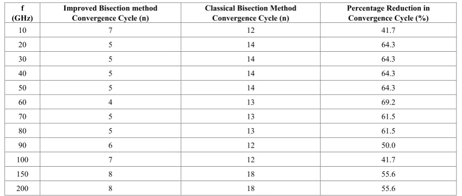
The result on convergence cycle versus frequency for the improved bisection method and the classical bisection method are shown in Table 5, Table 6 and Figure 5. As shown in Table 6, at 10 GHz, there is at least over 41 %
[image:9.595.69.528.354.544.2]Table 5. Improved bisection method: optimal path length, optimal fade depth, optimal path loss and convergence cycle versus frequency
f (GHz) Convergence Cycle Optimal Path Length Optimal Fade Depth Optimal Path loss
10 7 7.28 24.31 129.69
20 5 2.47 27.69 126.31
30 5 1.48 28.64 125.36
40 5 1.13 28.48 125.52
50 5 0.97 27.81 126.19
60 4 0.89 27.01 126.99
70 5 0.83 26.23 127.77
80 5 0.79 25.50 128.50
90 6 0.76 24.83 129.17
100 7 0.74 24.22 129.78
150 8 0.08 39.54 114.46
200 8 0.05 40.77 113.23
Figure 4. Improved bisection method: effect of frequency on optimal path length, initial path length and convergence cycle
[image:10.595.71.525.90.459.2] [image:10.595.116.482.482.733.2]Table 6. Improved bisection method and the classical bisection method: convergence cycle versus frequency
f
(GHz) Improved Bisection method Convergence Cycle (n) Classical Bisection Method Convergence Cycle (n) Percentage Reduction in Convergence Cycle (%)
10 7 12 41.7
20 5 14 64.3
30 5 14 64.3
40 5 14 64.3
50 5 14 64.3
60 4 13 69.2
70 5 13 61.5
80 5 13 61.5
90 6 12 50.0
100 7 12 41.7
150 8 18 55.6
200 8 18 55.6
5. Conclusions
An improved bisection algorithm for computing the optimal path length of wireless network link is presented. The performance of the algorithm is expressed in terms of the convergence cycle which is the minimum number of iterations at which the optimal path length is obtained. The performance of the improved bisection algorithm is compared with that of the classical bisection algorithm. In all, significant improvement in convergence cycle is achieved when the improve besection method is used.
REFERENCES
[1] Hasan, A. (2016). Numerical Study of Some Iterative Methods for Solving Nonlinear Equations. International Journal of Engineering Science Invention, 5(2), 01-10. [2] Hasan, A., & Ahmad, N. (2015). COMPARATIVE STUDY
OF A NEW ITERATIVE METHOD WITH THAT OF NEWTONS METHOD FOR SOLVING ALGEBRAIC AND TRANSCEDENTAL EQUATIONS.
[3] Khirallah, M. Q., & Hafiz, M. A. (2013). Solving system of nonlinear equations using family of jarratt methods. International Journal of Differential Equations and Applications, 12(2).
[4] Remani, C. (2012). Numerical methods for solving systems of nonlinear equations. Lakehead University, Thunder Bay, Ontario, Canada, 13.
[5] Suleiman, S. T. M. (2009). Solving System of Nonlinear Equations Using Methods in the Halley Class (Master's thesis, The University of Bergen).
[6] Lally, C. H. (2015). A faster, high precision algorithm for calculating symmetric and asymmetric $ M_ {T2} $. arXiv preprint arXiv:1509.01831.
[7] Ehiwario, J. C., & Aghamie, S. O. (2014). Comparative Study of Bisection, Newton-Raphson and Secant Methods
of Root-Finding Problems. IOSR Journal of Engineering (IOSRJEN), 4(04).
[8] Ait-Aoudia, S., & Mana, I. (2004). Numerical solving of geometric constraints by bisection: a distributed approach. International Journal of Computing & Information Sciences, 2(2), 66.
[9] Baskar, S., & Ganesh, S. S. (2005). Introduction to Numerical Analysis.
[10]Arsene, C. T. (2017). Operational decision support in the presence of uncertainties. arXiv preprint arXiv: 1701.04681. [11] Goodwin, D. L., & Kuprov, I. (2016). Modified
Newton-Raphson GRAPE methods for optimal control of spin systems. The Journal of chemical physics, 144(20), 204107.
[12] Mansouri, P., Asady, B., & Gupta, N. (2011). A novel iteration method for solve hard problems (nonlinear equations) with artificial bee colony algorithm. World Academy of Science, Engineering and Technology, 59, 594-596.
[13]Figueiredo, J. R., Santos, R. G., Favaro, C., Silva, A. F. S., & Sbravati, A. (2002). Substitution-Newton-Raphson method applied to the modeling of a vapour compression refrigeration system using different representations of the thermodynamic properties of R-134a. Journal of the Brazilian Society of Mechanical Sciences, 24(3), 158-168. [14]Intep, S. (2018). A Review of Bracketing Methods for
Finding Zeros of Nonlinear Functions. Applied Mathematical Sciences, 12(3), 137-146.
[15]Kobel, A., Rouillier, F., & Sagraloff, M. (2016, July). Computing Real Roots of Real Polynomials... and now for real! In Proceedings of the ACM on International Symposium on Symbolic and Algebraic Computation (pp. 303-310). ACM.
[image:11.595.66.530.90.287.2]equations. Mathematical Institute, University of Oxford. [18] Plagianakos, V. P., & Vrahatis, M. N. (2002). A Derivative
Free Minimization Method for Noisy Functions. In Combinatorial and Global Optimization (pp. 283-296). [19]Tanakan, S. (2013). A new algorithm of modified bisection
method for nonlinear equation. Applied Mathematical Sciences, 7(123), 6107-6114.
[20]Kestwal, M. C., Joshi, S., & Garia, L. S. (2014). Prediction of rain attenuation and impact of rain in wave propagation at microwave frequency for tropical region (Uttarakhand, India). International Journal of Microwave Science and Technology, 2014.
[21]Sarkar, S. K., & Kumar, A. (2007). Recent studies on cloud and precipitation phenomena for propagation characteristics over India. 92. 60. Nv; 84.40.-x.
[22]Ojo, J. S., Ajewole, M. O., & Sarkar, S. K. (2008). Rain rate and rain attenuation prediction for satellite communication in Ku and Ka bands over Nigeria. Progress in Electromagnetics Research, 5, 207-223.
[23]Kestwal, M. C., Joshi, S., & Garia, L. S. (2014). Prediction of rain attenuation and impact of rain in wave propagation at microwave frequency for tropical region (Uttarakhand, India). International Journal of Microwave Science and Technology, 2014.
[24]Zheng, L., Lu, N., & Cai, L. (2013). Reliable Wireless Communication Networks for Demand Response Control. IEEE Trans. Smart Grid, 4(1), 133-140.
[25]Zekavat, P. R., Moon, S., & Bernold, L. E. (2014). Performance of short and long range wireless communication technologies in construction. Automation in Construction, 47, 50-61.
[26]Xing, G., Lu, C., Zhang, Y., Huang, Q., & Pless, R. (2007). Minimum power configuration for wireless communication in sensor networks. ACM Transactions on Sensor Networks (TOSN), 3(2), 11.
[27]Emenyi M., Udofia K. M. & Amaefule O. C., (2017). Computation of Optimal Path Length for Terrestrial Line-of-sight Microwave links Using Newton–Raphson Algorithm. Software Engineering Volume 5, Issue 3, May 2017, Pages: 44-50
[28]Thorvaldsen, P., & Henne, I. (2014). Propagation measurements on a line-of-sight over-water radio link in Norway. Radio Science, 49(7), 531-548.
[29]Kestwal, M. C., Joshi, S., & Garia, L. S. (2014). Prediction of rain attenuation and impact of rain in wave propagation at microwave frequency for tropical region (Uttarakhand, India). International Journal of Microwave Science and Technology, 2014.
[30]Sulochana, Y., Chandrika, P., & Bhaskara Rao, S. V. (2017). Rainrate and rain attenuation statistics for different homogeneous regions of India. Indian Journal of Radio & Space Physics (IJRSP), 43(4-5), 303-314.