Munich Personal RePEc Archive
After the reforms: Determinants of wage
growth and change in wage inequality in
Vietnam: 1998-2008
Sakellariou, Chris and Fang, Zheng
September 2010
Online at
https://mpra.ub.uni-muenchen.de/27518/
1
After the Reforms: Determinants of Wage Growth and Change in Wage Inequality in Vietnam - 1998 -2008
Chris Sakellarioua* and Fang Zhenga
a
Division of Economics Humanities and Social Sciences Nanyang Technological University
Singapore
Abstract: The Vietnam ―renovation‖ reforms were implemented during the 1990s, but their full effect was only felt many years later. We present evidence on the developments in real wage growth and inequality in Vietnam from 1998 to 2008. For men, wage growth was underpinned by both increases in endowments of productive characteristics (mainly education) as well as changes in the wage structure (mainly associated with experience) and residual changes. For women, the wage structure effect was the main contributor to wage growth and the most important determinant was the change in the pattern of the returns to experience: younger, less experienced workers enjoyed a premium compared to more experience workers, reversing the previous, opposite pattern. Conventional measures of inequality as well as background analysis show that wage inequality decreased sharply through the 1990s until 2006, but increased subsequently. Over the entire 10-year period, wage inequality increased slightly and more so for women.
JEL codes: D33, J31, J42
Keywords: Wage inequality, counterfactual decompositions, Asia, Vietnam.
2
1. Introduction
During Vietnam’s central planning period (prior to 1986), policies were aimed at preserving
an egalitarian income distribution. Development during this period was accompanied by
misallocation of resources as a result of preserve incentives (see for example, Taylor 2004).
The Doi Moi (―renovation‖) reforms were initiated in 1986 and aimed at establishing a
market-based economy; however, these reforms actually started taking hold during the 1990s.
The consequences of the reforms were dramatic, with output per person increasing
significantly during the first decade of the reforms and the labor market particularly impacted.
Before the implementation of the reforms, public sector remuneration policy led to a
compression of earnings differentials across groups with different education qualifications.
The process of dismantling the old public sector wage system began in 19901. The role of
state-owned enterprises was lessened, salaries of public servants were set according to market
rates and the salary wage structure would reward public sector workers according to
education level, job responsibility and performance. Private firms were free to set wages
without government interference; for foreign ventures, however, an effective minimum wage
was set which was higher compared to the market wage and the minimum wage set for
domestic firms.2
The full impact of these reforms probably came only years later, since those hired
prior to 1994 were largely exempted (World Bank 1996). The implementation of these
reforms led to an increase in the demand for certain types of labor, particularly in trade and
services. This resulted in a shortage of high level technical experts, skilled technical workers,
administrative and managerial experts and researchers, among others (Nguyen et. al 1991).
1 Remuneration of public sector workers ceased to be based on length of service and jobs were no longer guaranteed for life (Hiebert 1993; Norlund 1993).
3
There are several studies, using various methodologies, for the United States, several
transition economies and some developing and Newly Industrialized Economies3. Studies in
this context are lacking for Vietnam (along with most countries in S.E. Asia), especially
studies using recent advances in methodology and recent data. Existing studies for Vietnam
include those by Nguyen et. al. (2006) who decomposed the urban-rural inequality from 1993
to 1998 using a quantile regression approach, Pham and Reilly (2007) who analysed the
gender pay gap along the earnings distribution from 1993 to 2002 and found a narrowing
gender pay gap, Gallup (2002) who derived conventional measures of inequality in the 1990s
and examined the contribution of wage employment to income growth and inequality and
Glewwe et. al. (2002) who examined changes in poverty and inequality in the 1990s and
found that poverty declined considerably during this period.
The objective of this paper is to establish the developments in wage growth and
inequality in Vietnam during the 1998-2008 period, that is the period from when reforms
started taking hold till when the Vietnamese economy and in particular the labor market had
been transformed. This involves comparison of wage distributions over time at quantiles. We
use Vietnam Living Standards and Vietnam Household Living Standards data from 1998 to
2008 and recent methodological advances which permit the identification of individual
contributors to over-time wage growth at different points of the wage distribution, in other
words implementing Oaxaca-Blinder decompositions at quantiles.
2. Methodology
2.1 Overview
In the last few years there has been an evolution and refinement of techniques used in
examining distributional issues, specifically in evaluating wage differentials between sub-
groups (and more generally the impacts of various programs) over the entire rage of the
4
earnings distribution. These new techniques were first used to analyse gender earning gaps
(for example, Albrecht et. al. 2003) and later to examine changes in wage distributions over
time, where the focal point is what contributes to the change in these distributions. This paper
implements recent advances in methodology, in particular a two-stage procedure proposed by
Firpo et. al. (2009; 2007), which allows the decomposition of changes or differences in wage
distributions and assessing the impact of explanatory variables on quantiles of the
unconditional wage distribution.
Oaxaca-Blinder decomposition techniques have been extensively utilized because
they not only allow decompositions of group differences or changes in mean wages, but also
permit further division of each component of the decomposition into individual contributions
of each covariate. Two drawbacks of these decomposition techniques are first, that the
contribution of each covariate is sensitive to the choice of the base group (see Oaxaca and
Ransom 1999) and second, the consistency of the estimates of the two decomposition
components depends on the linearity assumption (see Firpo et. al. 2007). Barsky et. al. (2002)
proposed a non-parametric reweighting approach along the lines of DiNardo et. al. (1996) to
deal with this problem. In the 1990s, procedures by Juhn et. al. (1993) and the re-weighting
procedure by DiNardo et. al. (1996) received attention. Later on, the decomposition at
quantiles method by Machado and Mata (2005)4 gained popularity. However, none of these
decomposition methodologies allowed for further subdivision of the characteristics
(composition) component into its constituent components.
Recently, Firpo et. al. (2009) proposed a new, computationally simple regression
method to evaluate the impact of changes in the distribution of explanatory variables (such as
education, union status, etc.) on quantiles of the unconditional (marginal) distribution of an
outcome variable (such as earnings). This method allows estimation of the effect of various
explanatory variables on the unconditional quantiles of an earnings variable.
5
2.2 Methodological Approach
The method used in this paper differs from the conditional quantile regression (Koenker and
Bassett 1978; Koenker 2005), as it is based on unconditional quantile regression
methodology. It involves estimating a regression of a transformation of the unconditional
quantile of the earnings variable on the explanatory variables (Re-centered Influence Function – RIF). This allows the estimation of standard partial effects (Unconditional Quantile Partial
Effects – UQPE). This regression method is then used to generate Oaxaca-Blinder
decompositions for quantiles of interest instead of the mean.
Consider differences in wage distributions between two groups, 1 and 0, in our case
one group at time 1 and the other at time 0. Let Y1i be the wage that would be paid to worker i
in period 1 and Y0i the wage that would be paid in period 0. In the case of Oaxaca-Blinder
decompositions at the mean, given the assumption of linearity:
Yti = Xiβt + εti, Ti=1, 0 and E[εti|Xi, T=t] = 0 (1)
To decompose the overall wage gap at the mean, Dµ, into wage structure and
composition effects we average over X, replacing the parameter vectors βt with their OLS
estimates and using the linearity assumption, we have:
Dµ = E[X|T = 1](β1−β0) + (E[X|T = 1] − E[X|T = 0])β0
= DµS + DµX (2)
When considering decompositions of changes in distributional statistics other than the
mean, most of the available techniques (for example, Juhn et. al. 1993; Donald et. al. 2000;
Machado and Mata 2005; Melly 2005), have the shortcoming that they don’t allow for further
dividing the wage structure and composition effect into the contributions of the individual
covariates. Firpo et. al. (2007; 2009) building on Firpo et. al. (2006) developed a
regression-based approach which allows for such a detailed decomposition.
Consider wage distributions for the 2 groups, with an interest in their differences.
6
depend on a vector of observed characteristics, Xi, as well as unobserved characteristics, εi,
depicted in the wage function:
Yti = gt(Xi, εi), t = 1, 0 (3)
Using the sample data (and assuming that (Y,T, X) have an unknown joint distribution),
one can identify the distributions: F1 for Y1|T = 1 and F0 for Y0|T = 0. One needs to also
identify the counterfactual distribution, FC for Y0|T = 1, that is the distribution that would
have prevailed if we have combined the wage structure of group 0 with the distribution of
characteristics of group 1. Comparing the wage distributions of the 2 groups by focusing on a
particular functional, ν (for example, the median), of the distributions the difference:
Dν= ν(F1) –ν(F0),
reflects the difference in wages (overall wage gap) measured in terms of the particular
distributional statistic chosen. Given that the composition of the two groups with respect to
characteristics, X, is generally different, the decomposition equation can then be written as:
Dν= [ν(F1) –ν(FC)] + [ν(FC) - ν(FC)] = DνS + DνX (4),
that is, as a sum of the wage structure and the composition effects.
In order to construct ν(FC) one needs to identify FC. For this as well as constructing
the composition effect component5 (DνX), a necessary assumption is that of conditional
independence (―ignorability‖). Firpo et. al. (2007) discuss why for the decomposition terms to
have the appropriate interpretation and for identifying the counterfactual distribution (FC),
besides this assumption the assumption of ―overlapping support‖ is also required. This
assumption requires that there is an overlap in observable characteristics across groups; this is
expected to be satisfied in our case, where we look at over-time changes in wage
distributions.
5 Since Dν
7
In identifying the parameters of the counterfactual distribution FC, and the two
components in equation (4), a reweighting approach is employed using three relevant
weighting functions: ω1(T), ω0(T) and ωC(T, X), which transform features of the marginal
distribution of Y into features of the conditional distribution of Y1 given T=1 and Y0 given
T=0, as well as the re-weighting function which transforms features of the marginal
distribution of Y into features of the counterfactual distribution of Y0 given T=1. In deriving
the re-weighting functions, the probability that a person belongs in group 1 conditional on X
(―propensity score‖) is derived from a logit regression.
While what has been described above allows the estimation of the 2 components of
the over-time changes in wage distributions, it does not permit estimation of the effect of
individual explanatory variables. This is accomplished using a recently proposed procedure
by Firpo et. al. (2009). This is a regression-based method that estimates the effect of
explanatory variables on the unconditional quantiles of the dependent variable (in our case
earnings). It involves estimating a regression of the rescaled (re-centered) influence function
of the unconditional quantile of earnings on the explanatory variables. This procedure
generates standard partial effects (unconditional quantile partial effects – UQPE).
Consider for example estimation of the direct effect of an increase in the proportion of
skilled workers6, p = Pr[X = 1], on a particular quantile of the wage distribution, where X
takes the value of 1 if the worker is skilled and 0 otherwise. In the case of quantile τ, using the
concept of the Influence Function (Hampel, 1974): IF(Y; qτ, FY) of a distributional statistic
ν(FY), which represents the influence of the individual observations on this statistic and
adding the statistic to the influence function, results in the Re-centered Influence Function
(RIF). Given that IF(Y; qτ, FY) is equal to (τ −1{Y ≤ qτ}) / fY (qτ), the RIF(Y; qτ, FY) is equal
to qτ + IF(Y; qτ, FY), while the conditional expectation of RIF(Y; qτ, FY) as a function of the
8
explanatory variables (i.e., E[RIF(Y; qτ, FY)|X=mτ(X)), is the unconditional quantile
regression model. Firpo et.al (2009) show that the average derivative of this regression
(E[mτ’(X)]) corresponds to the marginal effect on the unconditional quantile of a small
location shift in the distribution of covariates (holding everything else constant).
The decomposition components in equation (4) can now be re-written as:
DSqτ = E[m1qτ (X) | T=1] - E[mCqτ (X) | T=1]
DXqτ = E[mCqτ (X) | T=1] – E[m0qτ (X) | T=0]
Considering the linear projections (indexed by L) mLqτ (x):
mt,Lqτ (x) = xT. γtqτ and mC,Lqτ (x) = xT. γCqτ,
where: γtqτ = (E[X . XT | T = t]-1 . E[RIF(Yt; qτ, t) . X | T=t], t = 0,1 and:
γCqτ = (E[X . XT | T = 1]-1 . E[RIF(Yt; qτ, C) . X | T=1]
These linear projections of the true conditional expectation have an expected
approximation error of zero, hence:
E[mt,Lqτ (X) | T = t] = E[mtqτ (X) | T = t], t = 0, 1
E[mC,Lqτ (X) | T = 1] = E[mCqτ (X) | T = 1].
The decomposition is, then, rewritten as:
DSqτ = E[X | T = 1]T. (γtqτ - γCqτ) (5)
DXqτ = E[X | T = 1]T. γCqτ - E[X | T = 0]T. γ0qτ (6),
which is a generalization of the Oaxaca-Blinder decomposition through the projection of its
rescaled influence function onto the covariates. Note that equation (6) can be re-written as:
DXqτ = (E[X | T = 1] - E[X | T = 0])T. γ0qτ + Rqτ (6)’
where Rqτ is an approximation error. An error is involved since this regression based
procedure (as outlined in Firpo et.al. 2006) provides only a first-order approximation to the
composition effect. The approximation error can be estimated as the difference between the
estimate of the composition effect through re-weighting and the estimate obtained from the
RIF-9
regressions, an error component linked to a potential specification error is added, thus
changing the interpretation of the approximation error Rqτ.
Thus, using the RIF- regression estimates we can estimate the effect of a small change
in the distribution of X on a functional such as qτ, or a first-order approximation of a larger
change. Furthermore, Firpo et.al. (2006) show that in the case of quantiles, using a linear
specification in estimating the RIF-regressions yield very similar estimates to other
specifications, such as probit and logit.
3. Data and Estimation Samples
3.1 Summary Statistics
The data used draw on the household questionnaires from the 1997/8 Vietnam Living
Standard Surveys (VLSS) and the 2008 Vietnam Household Living Standard Survey (VHLSS
2008)7. The VLSS 1997/98 comprised of a sample of nearly 6,000 households, while the
VHLSS 2008 comprised of just over 9000 households From the wide range of questions
included in the household questionnaire, we utilize information on household member’s
characteristics such as age, gender, place of residence, education qualifications, as well as
employment information of workers employed for wages such as earnings, occupation and
major industry of employment.
Since this study focuses on wage and salary workers and excludes the self- employed
(for who there is no earnings information), the results are not representative of changes in
overall income or consumption inequality. However, one should look at changes in the
proportion of wage employment over the period examined. From the 1998 VLSS and 2008
VHLSS, the proportion of wage and salary employees in total non-farm employment was
approximately 48 % (21 % of all employed, including farm employment); this proportion
7
10
increased slightly to 49 % in 2008 (slightly less than 23 % of all employed). Therefore, the
proportion of wage and salary workers in non-farm and total employment did not change
substantially during the decade examined.
The dependent variable is the logarithm of the hourly wage, deflated to 1998 prices
using the CPI for Vietnam. The estimation samples include all those aged 15-65 who were
employed for wages in the public or public sector, including cooperatives, foreign enterprises
and joint ventures. Table A1 in the Appendix presents the mean characteristics of workers by
year and gender. Mean earnings grew strongly for both men and women and more so for
women. Real male wage earnings doubled, while female earnings increased by 140 %.
During the entire 1998-2008 period education endowments increased substantially; however,
there are significant gender differences. While the proportion of men with upper secondary
education increased significantly more than the corresponding proportion for women (46 vs.
14 % for upper secondary general), while the corresponding increase for tertiary
qualifications was 170 % for men vs. 110 % for women. Significant changes in the age
composition of wage earners are evident. Thus, the proportion of young, inexperienced
workers quadrupled for men and more than doubled for women; the proportion with 10 to 25
years of experience halved, while the corresponding proportion of older, more experience
workers doubled for men and nearly tripled for women. With respect to the occupational
composition of wage employment, the proportion of in professional and managerial
occupations more than doubled for men and increased by more than 50 % for women. Finally,
while primary sector employment remained approximately unchanged, the proportion of
wage earners in industry declined moderately, with a corresponding increase in the proportion
11
3.2 Conventional Measures of Inequality
One way to characterize inequality is to compute various summary measures of inequality.
Each measure of inequality has distinct properties8. Table 1 presents such measures, which
reveal a sharp decrease in wage inequality in Vietnam from 1992 to 2006 and a subsequent
rebound in the following years. Percentile ratios and their changes suggest that the inequality
decline applies mostly with reference to the bottom decile.
[Table 1 about here]
The over-time developments in measured wage inequality in Vietnam could be related
to the policy of imposing minimum wages and how it applies to various sectors. From 1993 to
1996, the minimum wage for all firms was 120,000 VND (about $12) per month, compared to
a minimum wage for firms with foreign ownership of $35 in Hanoi and HCM city and $30
elsewhere. Since 1997, the minimum monthly wage for unskilled labor applicable to both the
public and private sector was set at 144,000 VND per month; however, one important
difference is that in the public sector, the minimum wage is used as a base to calculate actual
salaries, which were set as a multiple of the minimum earnings; thus, an increase in the
minimum wage led automatically to an increase in public sector wages (see for example,
Belser, 2000).
While minimum wages in the domestic sector were modest for international standards
(less than 30 % of mean earnings), they have been revised consistently over the years to
450,000 VND in 2006 (870,000 VND for unskilled workers in the foreign invested sector in
Hanoi and Ho Chi Minh City) and 540,000 in 2008, all in nominal terms. At constant (1998)
prices, the minimum wage increased by 125 % between 1998 and 2006; however, the
corresponding increase between 1998 and 2008 was a little less than 100 %, because of high
inflation in recent years.
12
Chart 1 illustrates the changes in the real minimum wage and four inequality indices:
the Gini, along with the p90/p10, 90/50 and 50/10 percentile ratios from 1992 to 2008. The
developments over time, while not conclusive, are at least suggestive. The period of declining
inequality coincides with the sharp increase in the real minimum wage, until 2006. On the
other hand, after 2006 the real minimum wage declined, while all inequality indices increased
significantly.
[Chart 1 about here]
4. Estimation and Detailed Decomposition
4.1 RIF-Regressions
The unconditional quantile regression estimation consists of two steps. The first step is to
derive the re-centered influence function (RIF) of the dependent variable and the second step
involves estimating an OLS regression of the generated RIF variable on covariates. As shown
in Firpo et. al. (2009), the estimated coefficients are in fact unconditional partial effects of
small location shifts of the covariates.
Specifically, the RIF at quantiles is:
RIF(Y, qτ) = qτ+ [τ –I(Y ≤ qτ)/fY(qτ)],
where qτ can be estimated by the sample quantile and fY(.) can be estimated using Kernel
density. If the specification of the unconditional quantile regression is linear, the OLS
estimates of the coefficients are consistent estimators of the unconditional partial effects:
d(qτ)/d(X).
A well-known drawback of Oaxaca-Blinder decomposition techniques is that the
contribution of each covariate is sensitive to the choice of the base group (see for example,
Oaxaca and Ransom 1999). In this paper I apply the deviation contrast transform procedure
developed for use with such decompositions9. Applying the deviation contrast transformation
13
to the estimates before conducting the decomposition is one solution to this problem (see Yun
2005). The transformation procedure can be used to transform the coefficients of 0/1 dummy
variables so that they reflect deviations from the "grand mean" rather than deviations from the
reference category. Consequently, the modified coefficients will sum up to zero over all
categories.
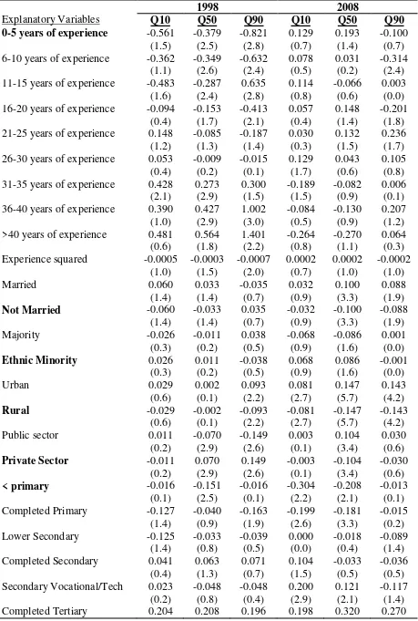
Tables A2 and A3 in the appendix report coefficients for all categories (including the
reference groups in the original model) with the constant modified accordingly. Some notable
over time changes include the sharp increase in wage premiums for professional occupations,
with a corresponding decrease in premiums for manual labor; the increase in the reward of
experience for younger, less experience workers, with a corresponding decrease in premiums
for older workers.
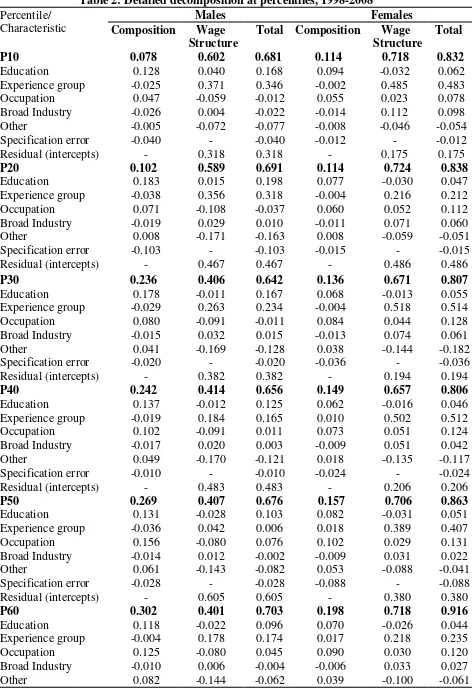
4.2 Detailed Decomposition Results
The outcome of the two-step procedure is estimates of the components of the total change in
log-wage, namely the composition and the coefficients (wage structure) component, as well as
the contribution of individual characteristics to these components and the total change (see
Table 2 and charts 2a-5b)10. The composition effect can be further divided into a part
explained by the vector of covariates in the model and a specification error; the error accounts
for the fact that a potentially incorrect linear specification was used in estimating the
RIF-regressions. Note that this does not affect the estimates of the two components (composition
and wage structure), which were derived using the re-weighting approach. However, one can
observe the size of the specification error and judge whether the method used (as proposed by
Firpo et. al. 2009; 2006) results in an accurate enough approximation of the problem at hand.
The wage structure effect can also be divided into the part explained by the RIF-regression
models and the residual change associated with change in intercepts.
14
Real earnings of both male and female wage employees showed strong growth over
the 10-year period examined. However, the pattern differs between men and women. First,
women enjoyed a higher increase in real earnings, with 2008 earnings higher by 2.3, 2.4 and
2.5 times compared to 1998 earnings at the 10th, 50th and 90th percentiles, respectively
(compared to about 2 times for men across the entire wage distribution). Second, the relative
magnitude of the two components differs substantially between genders. For men, the
composition (characteristics) component, while small at lower percentiles, increases at higher
points of the wage distribution and at the top exceeds the wage structure component. In other
words, over-time growth in earnings-generating characteristics play an important role in
shaping male wage growth over the 10-year period. For women, on the other hand, the
composition effect remains a small part of the total wage change at every point in the wage
distribution. The substantial wage structure component is the main contributor to the rear
wage growth of Vietnamese women. Furthermore, this component (as well as the total)
increases at higher points of the wage distribution. That is, at least for women, wage growth
has contributed to a moderate increase in wage inequality.
Turning to the contribution of individual covariates to the components of the overall
decomposition, the main components influencing total wage growth (column 3 in Table 2),
besides the component associated with change in intercepts11 are: experience group, region
and education. For men, the composition component is dominated by the growth in education
qualifications and to a lesser extent changes in occupational composition. The contributors to
the wage structure component, on the other hand, are: residual change (change in intercepts),
and changes in the reward to experience which contributed significantly to wage growth. The
effect of changes in the reward of experience is more evident at the bottom and at the very top
of the distribution. Changes associated with the reward to occupation as well as ―other‖
15
characteristics (marital status, ethnicity, urban/rural employment, sector of employment and
region) are towards decreasing earnings.
[Table 2 about here]
Women benefited less from the accumulation of education endowments because of a
slower growth in higher qualifications over the period examined compared to men; on the
other hand, changes in female occupational composition contributed positively to earnings
growth contrary to the case of men. The most important determinant of wage growth over the
period examined is the labor market reward by (potential) experience group, followed by
residual changes. Wage structure changes related to occupation and industry is also important,
with occupational wage structure changes benefiting women at lower parts of the wage
distribution.
To understand the effect of experience on wage growth in Vietnam, one needs to
examine tables A2 and A3; over time, the pattern of returns to experience group totally
changed at all points in the wage distribution. While in 1998 older, more experienced workers
enjoyed a substantial wage premium as compared to the youngest/least experienced group, by
2008 the opposite is the case. In 1998, for the median female worker, the return increases with
age/experience, peaking for the most experienced group. In 2008, on the other hand, the
highest return is for the most inexperienced group (0-5 years) and the lowest for the most
experienced (more than 40 years). The pattern varies slightly for other points in the
distribution; however the overall picture doesn’t change. Similar changes are observed for
men, with increasing returns for younger workers; however, the change in pattern is less
clear-cut.
In assessing the effect of wage growth on wage inequality over time in Vietnam, the
conclusion depends on what time period is examined. Presented evidence of wage growth
over the entire wage distribution from 1998 to 2008 suggests that wage inequality increased
1998-16
2006 period showed that wage inequality decreased drastically for both men and women.
Considering the evidence on changes in summary measures of inequality (Table 1), one can
conclude that wage inequality had been continuously decreasing from 1992 to 2006, but
increased sharply in subsequent years.
From the perspective of policy, policy makers are aware that the Vietnamese reforms
of the 1990s have the potential of increasing wage inequality, especially through changes in
the return to skill. Developments in wage inequality over the entire period since the early
1990s until 2008 suggest that interventions have been successful in ensuring that the benefits
of growth on wages are spread across all parts of the wage distribution. However,
developments over the 2006-2008 period (for example, increase in the Gini by 5.4 percentage
point or 15.5 % and in the Theil index by 9.7 percentage points or 42 %), may raise an alarm
and prompt further intervention, including a sharper revision of the nominal minimum wage in
Vietnam.
5. Conclusion
The Vietnam ―renovation‖ reforms, initiated in 1986 and implemented during the 1990s
aimed at establishing a market-based economy. The full impact of the reforms, especially in
the labor market, was felt only in recent years. As a result, the role of state-owned enterprises
was lessened, market forces were increasingly driving wages in both the private and public
sectors and rewards were increasingly based on education level, job responsibility and
performance.
In this paper we use recent advances in methodology and present evidence on the
developments in wage growth and inequality in Vietnam from 1998 to 2008, as well as the
contribution of individual covariates. Wage growth was strong over the 10-year period
examined, with real earnings doubling for men and more than doubling for women. For men,
17
wage growth, especially at higher points of the earnings distribution. For women, on the other
hand, changes in the wage structure shaped wage growth.
The composition component is dominated by the growth in education qualifications
and to a lesser extent changes in occupational composition. Women benefited less from the
accumulation of education endowments compared to men, because of a slower growth in
higher qualifications over the period examined. Besides residual changes, the most important
component influencing wage growth through the wage structure effect for both men and
women is associated with experience. This is the result of drastic over-time changes in the
patter of returns to experience, especially for women; by 2008, younger workers enjoy the
highest returns to labor market experience, reversing the opposite earlier pattern.
Finally, assessing changes in wage inequality hinges on the length of period examined.
Over the whole 10-year period, wage inequality slightly increased; however, background
analysis as well as the developments in summary inequality indices shows that wage
inequality was decreasing continuously until 2006, and increased thereafter. The evidence
presented is at least suggestive of a relationship between the real minimum wage and wage
18
References
Barsky, R., J. Bound, K. Charles and J. Lupton, ―Accounting for the Black-White Wealth Gap:
A Nonparametric Approach.‖ Journal of the American Statistical Association, 97(459): 663-673, 2002.
Belser, P., ―Vietnam, on the road to Labor-Intensive growth?‖ WPS 2389, the World Bank, East Asia and Pacific Region, Vietnam country office, July 2000.
Bourguignon, F., M. Fournier, and M. Gurgand, ―Fast Development with a Stable Income Distribution.‖ Review of Income and Wealth, 47 (2): 139-163, 2001.
DiNardo, J., M. Fortin and T. Lemieux, ―Labor Market Institutions and the Distribution of Wages, 1973-1992: A Semiparametric Approach.‖ Econometrica, 64: 1001-1044, 1996.
Donald, S. G., D. A. Green and H. J. Paarsch, ―Differences in Wage Distributions between Canada and the United States: An Application of a Flexible Estimator of Distribution Functions
in the Presence of Covariates Source.‖ The Review of Economic Studies, 67(4): 609-633, 2000.
Fields, G. S., ―Accounting for Income Inequality and its Change: A New Method with
Application to U.S. Earnings Inequality.‖ In Solomon W. Polacheck (Ed.), Research in Labor
Economics vol 22: Worker Well-Being and Public Policy. Oxford: JAI pp 1-38.2003.
________ and G. Yoo, ―Falling Labour Income Inequality in Korea's Economic Growth: Patterns and Underlying Causes." Review of Income and Wealth, 46(2): 139-159, 2000.
________ N. Fortin, and T. Lemieux, ―Decomposing Wage Distributions Using Recentered
Influence Function Regressions.‖ Unpublished Manuscript, University of British Columbia, 2007.
________ ―Decomposing Wage Distributions Using Recentered Influence Function
Regressions.‖ Working Paper, University of British Columbia, 2007.
________ ―Unconditional Quantile Regressions.‖ Econometrica, 77 (3): 953-973, 2009
Gallup, J. L., ―The Wage Labor Market and Inequality in Vietnam in the 1990s.‖ World Bank Policy Research Working Paper No. 2896, Washington, D.C., 2002.
Glewwe, P., M. Gragnolati, and H. Zaman, ― Who Gained from Vietnam’s Boom in the
1990s?‖ Economic Development anc Cultural Change, 50(4), 773—792, 2002.
Gosling, A., S. Machin, and C. Meghir, ―The changing Distribution of Male Wages in the U.K.‖ Review of Economic Studies, 67: 635-686, 2000.
Hampel, F. R., ―The Influence Curve and its Role in Robust Estimation.‖ Journal of the American Statistical Association, 60: 383-393, 1974.
19
Juhn, C., K. Murphy and B. Pierce, ―Wage Inequality and the Rise in Returns to Skill.‖ The Journal of Political Economy, 101: 410-442, 1993.
Koenker, R. and G. Bassett, ―Regression at Quantiles.‖ Econometrica, 46: 33-50,1978.
Koenker, R., Quantile Regression. New York, Cambridge University Press, 2005.
Lukyanova, A., ―Wage Inequality in Russia: 1994-2003.‖ Economic Research Network, Russia and CIS Working Paper no. 06/03, Moscow, 2006.
Machado, J.A.F and J. Mata, ―Counterfactual Decomposition of Changes in Wage
Distributions Using Quantile Regressions.‖ Journal of Applied Econometrics, 20: 445-65, 2005.
Melly, B., ―Decomposition of Differences in Distribution Using Quanitle Regressions.‖
Labour Economics, 12: 577-90, 2005.
Meng, X., ―Economic Restructuring and Income Inequality in Urban China.‖ Review of Income and Wealth, 50(3): 357-79, 2004.
Nguyen, T. L., B. T. Nguyen, Vu Binh Cu, V. T. Nguyen and M. Godfrey, ―Human
Resources Development.‖ In Ronnas and Orjan Sjoberj (Eds), Socio-economic Development in Vietnam, 1991.
Nguyen, B. T., J. Albrecht, S. Vroman, and M. D. Westbrook, ―A Quantile Regression Decomposition of Urban-Rural Inequality in Vietnam.‖ Economics and Research Department, Asian Development Bank, Manila, 2006.
Norlund, I., ―The Creation of a Labour Market in Vietnam: Legal Framework and Practices.‖ In C. A. Thayer and D. G. Marr (Eds), Vietnam and the Rule of Law. Political and Social Change Monograph No. 19, Australian National University, Cambera, 1993.
Oaxaca,R L. and M. R. Ransom, ―On Discrimination and the Decomposition of Wage
Differentials,‖ Journal of Econometrics, 61(1): 5-21, 1994.
_________ ―Identification in Detailed Wage Decompositions.‖ Review of Economics and Statistics,81(1): 154–157, 1999.
Pham, H. T. and B. Reilly., ―The Gender Pay Gap in Vietnam, 1993-2002: A Quantile
Regression Approach.‖ MPRA Paper N0. 6475, 2007.
Taylor, P., ―Introduction: Social inequality in a socialist state.‖ In P. Taylor (ed): Social inequality in Vietnam and the challenges to reform, Institute of Southeast Asia Studies, Singapore, 2004.
World Bank, Vietnam Education Financing Sector Study. Report N0. 15925-VN, Washington, D.C., 1996.
Yun, M. S., ―A Simple Solution to the Identification Problem in Detailed Wage
20
Table 1: Change in Various Inequality Measures over Time Inequality measure 1992 1998 2002 2006 2008 % change
1998-06
% change 1998-08
% change 2006-08
Relative Mean Deviation Coefficient of Variation Standard Deviation of logs Gini Coefficient
Theil Entropy Measure Percentile Ratios p90/p10
p90/p50 p75/p25 p50/p10
0.303 1.42 0.756 0.428 0.396
6.00 2.40 2.61 2.50
0.282 0.981 0.715 0.396 0.298
5.60 2.40 2.34 2.33
0.263 0.964 0.709 0.377 0.274
5.36 2.12 2.27 2.53
0.249 0.903 0.620 0.349 0.231
4.54 2.27 2.14 2.00
0.288 1.172 0.716 0.403 0.328
5.59 2.51 2.49 2.23
-11.7 -8.0 -13.3 -11.9 -22.5
-18.9 -5.4 -8.5 -14.2
2.1 19.5
0.1 1.8 10.1
-0.2 4.6 6.4 -4.3
15.7 29.8 15.5 15.5 42.0
23.1 10.6 16.4 11.5
21
Table 2:Detailed decomposition at percentiles, 1998-2008
Percentile/ Characteristic
Males Females
Composition Wage Structure
Total Composition Wage Structure Total P10 Education Experience group Occupation Broad Industry Other Specification error Residual (intercepts)
0.078 0.602 0.681 0.114 0.718 0.832
0.128 -0.025 0.047 -0.026 -0.005 -0.040 - 0.040 0.371 -0.059 0.004 -0.072 - 0.318 0.168 0.346 -0.012 -0.022 -0.077 -0.040 0.318 0.094 -0.002 0.055 -0.014 -0.008 -0.012 - -0.032 0.485 0.023 0.112 -0.046 - 0.175 0.062 0.483 0.078 0.098 -0.054 -0.012 0.175 P20 Education Experience group Occupation Broad Industry Other Specification error Residual (intercepts)
0.102 0.589 0.691 0.114 0.724 0.838
0.183 -0.038 0.071 -0.019 0.008 -0.103 - 0.015 0.356 -0.108 0.029 -0.171 - 0.467 0.198 0.318 -0.037 0.010 -0.163 -0.103 0.467 0.077 -0.004 0.060 -0.011 0.008 -0.015 - -0.030 0.216 0.052 0.071 -0.059 - 0.486 0.047 0.212 0.112 0.060 -0.051 -0.015 0.486 P30 Education Experience group Occupation Broad Industry Other Specification error Residual (intercepts)
0.236 0.406 0.642 0.136 0.671 0.807
0.178 -0.029 0.080 -0.015 0.041 -0.020 - -0.011 0.263 -0.091 0.032 -0.169 - 0.382 0.167 0.234 -0.011 0.015 -0.128 -0.020 0.382 0.068 -0.004 0.084 -0.013 0.038 -0.036 - -0.013 0.518 0.044 0.074 -0.144 - 0.194 0.055 0.514 0.128 0.061 -0.182 -0.036 0.194 P40 Education Experience group Occupation Broad Industry Other Specification error Residual (intercepts)
0.242 0.414 0.656 0.149 0.657 0.806
0.137 -0.019 0.102 -0.017 0.049 -0.010 - -0.012 0.184 -0.091 0.020 -0.170 - 0.483 0.125 0.165 0.011 0.003 -0.121 -0.010 0.483 0.062 0.010 0.073 -0.009 0.018 -0.024 - -0.016 0.502 0.051 0.051 -0.135 - 0.206 0.046 0.512 0.124 0.042 -0.117 -0.024 0.206 P50 Education Experience group Occupation Broad Industry Other Specification error Residual (intercepts)
0.269 0.407 0.676 0.157 0.706 0.863
0.131 -0.036 0.156 -0.014 0.061 -0.028 - -0.028 0.042 -0.080 0.012 -0.143 - 0.605 0.103 0.006 0.076 -0.002 -0.082 -0.028 0.605 0.082 0.018 0.102 -0.009 0.053 -0.088 - -0.031 0.389 0.029 0.031 -0.088 - 0.380 0.051 0.407 0.131 0.022 -0.041 -0.088 0.380 P60 Education Experience group Occupation Broad Industry Other
0.302 0.401 0.703 0.198 0.718 0.916
22 Specification error Residual (intercepts) -0.008 - - 0.463 -0.008 0.463 -0.013 - - 0.563 -0.013 0.563 P70 Education Experience group Occupation Broad Industry Other Specification error Residual (intercepts)
0.336 0.383 0.719 0.162 0.758 0.920
0.108 0.020 0.106 -0.006 0.083 0.024 - -0.006 0.140 -0.062 0.014 -0.074 - 0.371 0.102 0.160 0.044 0.008 0.009 0.024 0.371 0.071 0.010 0.087 -0.004 0.022 -0.023 - -0.008 0.430 -0.021 0.031 -0.154 - 0.480 0.063 0.440 0.066 0.027 -0.132 -0.023 0.480
P80 0.360 0.348 0.708 0.185 0.787 0.972
Education Experience group Occupation Broad Industry Other Specification error Residual (intercepts) 0.136 0.013 0.103 -0.001 0.066 0.042 - -0.015 0.133 -0.092 0.008 -0.078 - 0.393 0.121 0.146 0.011 0.007 -0.012 0.042 0.393 0.072 0.020 0.120 -0.008 0.031 -0.049 - -0.015 0.588 -0.090 0.018 -0.056 - 0.343 0.057 0.608 0.030 0.010 -0.025 -0.049 0.343 P90 Education Experience group Occupation Broad Industry Other Specification error Residual (intercepts)
0.409 0.308 0.717 0.103 0.829 0.932
23
Source: author’s calculations.
0 20 40 60 80 100 120 140 160 180 200
1992 1998 2002 2004 2006 2008
Chart 1: Real Min. Wage and Inequality Indices Over Time:
1992-2008
Real Minimum Wage
Gini
90/10
90/50
24
[image:25.595.69.526.107.698.2]Appendix
Table A1: Summary Statistics by Year: Male Wage Employees 15-65 Years (%)
Characteristic 1998 2008
Male Female Male Female
Hourly wage, 1998 prices (Viet Dong)
0-5 years of experience
6-10 years of experience 11-15 years of experience 16-20 years of experience 21-25 years of experience 26-30 years of experience 31-35 years of experience 36-40 years of experience >40 years of experience Married Not Married Majority Ethnic Minority Urban Rural Public sector Private Sector < Primary education
Completed Primary Lower Secondary Completed Secondary Secondary Vocational/Tech Completed Tertiary Manager/Official Professional/Assoc. Professional Service/Sales Skilled labor Unskilled labor Primary sector Industry Trade/Services Red River Delta North
Central South-East
Mekong River Delta
25
Table A2: Transformed coefficients from RIF-Regressions on the Log of hourly Wage -
Males
Explanatory Variables
1998 2008
Q10 Q50 Q90 Q10 Q50 Q90
0-5 years of experience
6-10 years of experience
11-15 years of experience
16-20 years of experience
21-25 years of experience
26-30 years of experience
31-35 years of experience
36-40 years of experience
> 40 years of experience
26 Completed Tertiary Manager/Official Professional Service/Sales Skilled labor Unskilled labor Primary sector Industry Trade/Services
Red River Delta
North
Central
South-East
Mekong River Delta
Constant (2.2) 0.397 (3.4) -0.279 (2.0) 0.013 (0.1) -0.190 (1.4) 0.122 (1.6) 0.334 (3.9) -0.095 (1.4) 0.170 (3.4) -0.075 (1.4) -0.360 (5.0) -0.134 (1.9) 0.145 (2.8) 0.196 (4.8) 0.151 (2.5) -0.052 (0.2) (0.1) 0.306 (5.4) -0.109 (2.1) -0.003 (0.1) -0.111 (2.4) 0.130 (3.5) 0.092 (2.4) 0.059 (1.9) 0.018 (0.6) -0.077 (2.9) -0.220 (6.9) -0.226 (6.3) 0.022 (0.6) 0.266 (10.0) 0.159 (4.9) 0.994 (8.4) (0.6) 0.597 (4.5) -0.040 (0.4) 0.037 (0.5) -0.195 (2.5) 0.129 (1.7) 0.069 (1.0) 0.056 (0.8) -0.022 (0.4) -0.034 (0.6) -0.234 (4.8) -0.143 (2.4) -0.132 (2.3) 0.376 (5.7) 0.133 (2.0) 2.19 (9.9) (2.9) 0.224 (2.8) -0.069 (0.5) 0.202 (2.7) -0.281 (1.8) 0.175 (2.6) -0.026 (0.3) -0.110 (1.7) 0.214 (4.2) -0.104 (1.8) -0.122 (1.9) -0.065 (0.9) -0.037 (0.5) 0.210 (4.5) 0.014 (0.2) 0.231 (0.9) (2.5) 0.314 (5.8) -0.008 (0.1) 0.410 (8.9) -0.204 (2.6) -0.054 (1.0) -0.144 (2.7) 0.000 (0.0) 0.076 (2.2) -0.075 (1.8) -0.066 (1.7) -0.056 (1.1) 0.005 (0.1) 0.144 (3.2) -0.037 (0.7) 1.52 (9.8) (0.2) 0.358 (2.9) 0.069 (0.6) 0.300 (4.0) -0.135 (1.8) -0.107 (1.3) -0.128 (2.2) 0.097 (1.6) -0.063 (1.1) -0.033 (0.4) 0.030 (0.4) -0.144 (2.1) -0.199 (3.0) 0.435 (4.8) -0.121 (1.7) 2.41 (12.4)
N 1,852 1,547
27
Table A3: Transformed coefficients from RIF-Regressions on the Log of hourly Wage - Females
Explanatory Variables
1998 2008
Q10 Q50 Q90 Q10 Q50 Q90
0-5 years of experience
6-10 years of experience
11-15 years of experience
16-20 years of experience
21-25 years of experience
26-30 years of experience
31-35 years of experience
36-40 years of experience
>40 years of experience
28 Manager/Official Professional Service/Sales Skilled labor Unskilled labor Primary sector Industry Trade/Services
Red River Delta
North
Central
South-East
Mekong River Delta
Constant (1.7) -0.163 (0.5) 0.341 (2.8) 0.095 (0.5) -0.107 (0.9) -0.166 (1.1) 0.303 (2.9) 0.173 (2.6) -0.475 (4.4) -0.271 (2.4) -0.264 (2.5) 0.147 (1.7) 0.316 (5.2) 0.072 (0.8) 0.510 (1.3) (3.1) 0.014 (0.1) 0.233 (4.5) -0.003 (0.0) -0.135 (2.3) -0.109 (2.0) 0.139 (3.1) 0.050 (1.2) -0.188 (5.1) -0.106 (2.3) -0.231 (5.5) -0.002 (0.0) 0.203 (5.8) 0.136 (3.2) 1.11 (7.6) (1.3) -0.153 (0.9) 0.573 (5.1) -0.219 (2.0) -0.075 (0.6) -0.126 (1.3) 0.167 (2.1) -0.067 (0.8) -0.099 (1.2) 0.014 (0.2) -0.211 (3.1) -0.149 (2.4) 0.230 (3.1) 0.116 (1.4) 2.143 (7.3) (3.1) -0.112 (0.9) 0.252 (4.4) -0.159 (1.3) 0.144 (2.1) -0.125 (1.4) -0.118 (2.0) 0.198 (4.4) -0.080 (1.5) -0.196 (3.2) -0.215 (3.2) 0.147 (2.4) 0.318 (7.2) -0.054 (0.7) 0.647 (3.3) (5.4) 0.023 (0.3) 0.512 (10.2) -0.112 (1.4) -0.206 (3.6) -0.217 (3.5) 0.005 (0.1) 0.102 (2.7) -0.107 (2.3) -0.110 (2.5) -0.205 (4.3) 0.040 (0.8) 0.267 (5.7) 0.008 (0.2) 1.40 (9.7) (2.2) 0.368 (3.1) 0.375 (4.9) -0.059 (0.5) -0.350 (4.5) -0.335 (5.1) 0.064 (1.4) 0.126 (2.0) -0.191 (2.4) 0.002 (0.0) -0.148 (2.2) -0.031 (0.4) 0.221 (2.9) -0.044 (0.6) 2.641 (19.4)
N 1,207 1,582
29 0
0.2 0.4 0.6 0.8 1 1.2
P10 P20 P30 P40 P50 P60 P70 P80 P90 Chart 2b: Decomposition of Changes in Log-Wage - Females
Composition Wage Structure Total
-0.15 -0.1 -0.05 0 0.05 0.1 0.15 0.2 0.25 0.3
P10 P20 P30 P40 P50 P60 P70 P80 P90 Chart 3b: Components of the
Composition Effect - Females
Total Explained Spec. Error
-0.2 -0.1 0 0.1 0.2 0.3 0.4 0.5
P10 P20 P30 P40 P50 P60 P70 P80 P90 Chart 3a: Components of the
Composition Effect - Males
Total Explained Spec. Error
0 0.1 0.2 0.3 0.4 0.5 0.6 0.7 0.8
P10 P20 P30 P40 P50 P60 P70 P80 P90 Chart 2a: Decomposition of Changes in Log-Wage - Males
30 0
0.1 0.2 0.3 0.4 0.5 0.6 0.7 0.8 0.9
P10 P20 P30 P40 P50 P60 P70 P80 P90 Chart 4b: Components of the
Wage Structure Effect - Females
Total Explained Residual (Intercepts)
-0.3 -0.2 -0.1 0 0.1 0.2 0.3 0.4 0.5 0.6 0.7
P10 P20 P30 P40 P50 P60 P70 P80 P90 Chart Ab: Contributors to Total
Log-Wage change - Females
Education Experience
Occupation Industry
Other -0.3
-0.2 -0.1 0 0.1 0.2 0.3 0.4 0.5 0.6 0.7
P10 P20 P30 P40 P50 P60 P70 P80 P90 Chart 4a: Components of the
Wage Structure Effect - Males
Total Explained Residual (Intercepts)
-0.2 -0.1 0 0.1 0.2 0.3 0.4 0.5
P10 P20 P30 P40 P50 P60 P70 P80 P90 Chart 5a: Contributors to Total
Log-Wage change - Males
Education Experience
Occupation Industry