http://dx.doi.org/10.4236/acs.2016.63035
How to cite this paper: Balarabe, M., Abdullah, K., Nawawi, M. and Khalil, A.E. (2016) Monthly Temporal-Spatial Variability and Estimation of Absorbing Aerosol Index Using Ground-Based Meteorological Data in Nigeria. Atmospheric and Climate Sciences, 6, 425-444. http://dx.doi.org/10.4236/acs.2016.63035
Monthly Temporal-Spatial Variability and
Estimation of Absorbing Aerosol Index
Using Ground-Based Meteorological
Data in Nigeria
Mukhtar Balarabe
1,2*, Khiruddin Abdullah
1, Mohd Nawawi
1, Amin Esmail Khalil
1 1School of Physics, University Sains Malaysia, Pulau Pinang, Malaysia2Hassan Usman Katsina Polytechnic, Katsina, Nigeria
Received 6 April 2016; accepted 5 July 2016; published 8 July 2016
Copyright © 2016 by authors and Scientific Research Publishing Inc.
This work is licensed under the Creative Commons Attribution International License (CC BY).
http://creativecommons.org/licenses/by/4.0/
Abstract
The objective of this work is to analyze the temporal and spatial variability of the monthly mean aerosol index (AI) obtained from the Total Ozone Mapping Spectrometer (TOMS) and Ozone Mon-itoring Instrument (OMI) in comparison with the available ground observations in Nigeria during 1984-2013. It also aims at developing a regression model to allow the estimation of the values of AI in Nigeria based on the data from ground observations. TOMS and OMI data are considered and treated separately to provide continuity and consistency in the long-term data observations, to-gether with the meteorological variable such as wind speed, visibility, air temperature and rela-tive humidity that can be used to characterize the dust activity in Nigeria. The results revealed a strong seasonal pattern of the monthly distribution and variability of absorbing aerosols along a north to south gradient. The monthly mean AI showed higher values during the dry months (Har-mattan) and lower values during the wet months (Summer) in all zones. From December to Feb-ruary, higher AI values are observed in the southern region, decreasing progressively towards the north, while during March-October, the opposite pattern is observed. The AI showed clear maxi-mum values of 2.06, 1.93, and 1.87 (TOMS) and 2.32, 2.27 and 2.24 (OMI) in the month of January and minimum values in September over the north-central, southern and coastal zones, while show-ing maximum values of 1.76 (TOMS) and 2.10 (OMI) durshow-ing March in the Sahel. New empirical al-gorithms for predicting missing AI data were proposed using TOMS data and multiple linear re-gression, and the model co-efficient was determined. The generated coefficients were applied to another dataset for cross-validation. The accuracy of the model was determined using the
coeffi-cient of determination R2 and the root mean square error (RMSE) calculated at the 95%
confi-dence level. The AI values for the missing years were retrieved, plotted and compared with the *
measured monthly AI cycle. It is concluded that the meteorological variables can significantly ex-plain the AI variability and can be used efficiently to predict the missing AI data.
Keywords
Aerosol Index, Nigeria, Relative Humidity, Temperature, Visibility
1. Introduction
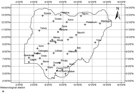
Dust aerosol has become the most abundant aerosol type in the atmospheric column worldwide [1]. It is the most significant source of atmospheric aerosol in the western Sahel (including Nigeria) [2]. This is due to the location of Nigeria in Sub-Sharan West Africa [3]. Nigeria is located between the latitudes 4˚ - 14˚ and the longitudes 3˚- 15˚E, and sandwiched between the Gulf of Guinea to the south and Sahel belt of West Africa to the north. Ap-proximately 12 of the 36 states of Nigeria to the north fall entirely or partially within the Sahel [3]. The Sahel is close to the Sahara Desert, and they are described as the most important global dust source regions [4]. Aerosols are transported regularly from these sources across Nigeria towards the Atlantic Ocean. The intensity of dust transport is a seasonal phenomenon due to the existence of the intertropical convergence zone (ITCZ), which serves as a moving boundary between the dry north-easterly winds (tropical continental air mass) and the moist south-westerly winds (tropical maritime air mass). These two air masses usually originate from the high- pressure belt located north of the Tropic of Cancer and the high-pressure belt located off the coast of Namibia. The interplay between the two air masses gives rise to two distinct and well-defined seasons in Nigeria, namely, the dry seasons (dust-laden), also known as Harmattan, and the summer (wet or rainy season). The dry season in the southern part of Nigeria occurs between November and February, whereas the wet season occurs between March and October. In the northern zones, the dry season occurs between November and May, while the wet season takes place between June and September [5]. During the Harmattan season, the entire country experiences large quantities of dust and smoke from biomass burning that is transported by the prevailing north-east trade winds. During this period, favorable weather conditions also contribute to more dust emission and distribution in the at-mosphere. This is in addition to anthropogenic activities that normally arise from high energy demands and increase the pressure on land for agricultural purposes and infrastructure. Based on these, Anuforom et al.[3] described Ni-geria as one of the heavily aerosol-laden regions of West Africa, where aerosol studies are of great interest.
The period of dust transport over Nigeria is characterized by lower than normal temperatures in the early morning and night time, and hotter temperature during the day time. The most observable of dust aerosol effect across Nigeria is visibility reduction resulting from scattering and absorption of solar radiation by suspended particles in the atmosphere. During low-visibility events, many flight operations are suspended or delayed, which leads to a significant economic loss for Nigeria [6]. It has been recognized that dust affects not only the regional but also the global climate system [3], respiratory tracts, and cloud microphysical properties [1]. Dust aerosol also affects the cooling and heating rates at different latitudes [7], regional air quality, and human health [8]. As a result of these numerous effects of dust aerosol, it has become an essential parameter in atmospheric aerosol studies that requires constant monitoring and evaluation. Therefore, there is considerable interest at the global, regional and local levels in climate variability and the distribution of aerosol, including dust [1][9][10] [11]. For instance, Pal et al.[11] analyzed long-term Lidar and radiometric data to investigate the monthly time series of the aerosol distribution at different altitudes as well as within the atmospheric boundary layer using a wavelet-based spectral analysis. This is aimed at investigating different periodicities present in the long-term dataset over India. However, the quantification of the dust aerosol effects on the climate, solar radiation, envi-ronment, and health are associated with large uncertainty due to the variety of aerosol sources, complex interac-tions with other aerosols, and solar radiation, as well as clouds and varying trend patterns [1][9].
problems of spatial density and limitations due to the short time of aerosol observations, the use of Aerosol In-dex (AI) data from the TOMS and OMI is necessary. The AI provides a qualitative measure of the amount of UV-absorbing aerosol, which is mainly biomass burning and dust [14]. Although AI does not quantify the actual dust concentration, many papers in the literature have used it as a proxy for the dust aerosol concentration [4], which represents the presence of dust in the atmosphere [1]. This includes a surface-based study in tropical At-lantic, which shows a significant correlation between the mineral dust concentration measured at the surface and the TOMS AI [15]. The AI is therefore increasingly utilized in soil dust monitoring [3]. TOMS and OMI detect the presence of both UV-absorbing aerosols such as dust and smoke and non-absorbing aerosols such as sulfate and sea salt [4]. The positive AI indicates the dominance of UV-absorbing aerosol [16], and the negative values indicate non-absorbing aerosol [14]. In line with this, some authors have the opinion that dust represents the clearest absorption signature [17].
Despite the continuous use of AI in studying dust phenomena, the use of the TOMS data for long-term study is difficult due to the large gap of missing data from April 1993 to August 1996 and early calibration problems detected in the TOMS Earth-probe signal after July 2000 [18]. These leave gaps in our long-term TOMS AI data record and can create challenges in aerosol studies associated with dust. These gaps are visible in the previous study of Balarabe et al.[19]. To overcome this problem, this paper has a dual focus. One goal is to explore the temporal variations and spatial distribution of the monthly mean AI obtained from TOMS and OMI in relation to the spatial distribution of ground meteorological data in Nigeria during 1984-2013. The other is to develop AI monthly regression models that allow the estimation of the missing values of AI observations for Nigeria, with potential global applications. The models are developed based on four selected types of meteorological data from ground observations, namely, i) wind speed, ii) visibility, iii) temperature, and iv) relative humidity. The AI prediction models based on these measurements are necessary so that missing AI values can be estimated as long as these meteorological parameters are available.
The study of the temporal variations and spatial distribution of the monthly AI in relation to the meteorologi-cal parameters is significant in Nigeria because although dust aerosol is the dominant aerosol type over Sub- Saharan West Africa, the extent of its monthly variability in space and time and its relationship with meteoro-logical parameters has not been exhaustively studied at a regional scale. The study of this phenomenon will in-crease our understanding of dust activity in Nigeria. Regional studies on the AI distribution have been conducted at different locations such as India [9], Greece [14], and Pakistan [16]. The authors revealed that the spatial dis-tribution in AI is related to the Saharan dust events, pollution transport and variations in meteorology. Under-standing the AI distribution at a local scale is therefore significant. The new proposed models are also signifi-cant in this study because they enable the development of a long-term AI data base for better monitoring and understanding of absorbing aerosol trends (spatial and temporal) and variability over an extended period. It can also be used for various meteorological applications, the aviation industry, and air pollution studies. This study is the first of its kind that analyzes the temporal and spatial variability of the monthly mean AI from TOMS and OMI, as well as its relationship with available observations of ground meteorological data in Nigeria. It is also the first based on available literature to use multiple linear regression for AI prediction, taking into account the meteorology of the study area. However, a similar approach was used by Fuyi et al.[20] to develop a model for AOD retrieval. It is important to note that TOMS and OMI data are used and treated separately to provide con-tinuity and consistency in the long-term data observation, while meteorological parameters such as wind speed and visibility are used to characterize the dust activity.
different zones of Nigeria [19]. The relationship between the OMI AI and latitude over Greece was studied by Kaskoutis et al.[15]. Although only the visibility, precipitation and latitude were considered in the previous li-terature to model AI, the need to consider other meteorological variables has been noted by Salman et al.[16] and Fuyi et al.[20].
2. Data and Methodology
2.1. TOMS Aerosol Index Data
The TOMS instrument flew in space as an orbiting satellite from November 1978 to August 2005 on four dif-ferent platforms: Nimbus 7 polar-orbiting from November 1978 to May 1993, Meteor 3 satellite from August 1991 to December 1994 [22], EP/TOMS from July 2, 1996, and ADEOS/TOMS in August 1996. The second TOMS instrument (EP/TOMS) operated on the Russian Meteor and was a modified version of the Nimbus 7. This was a sun-synchronous low-altitude orbit, designed for better detection of absorbing aerosols before ADEOS/TOMS was launched into a higher orbit with a spatial resolution similar to that of Nimbus 7/TOMS.
The fact that the intensity of aerosols effect on atmospheric process is more in UV band, Aerosol Index (AI) is defined as the qualitative indicator of the presences of both absorbing aerosol such as dust and smoke and non-absorbing aerosol such as sulfate and sea-salt in the UV-range [22]. We downloaded the monthly sun- synchronous Nimbus 7/TOMS data from 1984-1993 and EP/TOMS from 1996-2000 from the NASA website
ftp://jwocky.gsfc.nasa.gov/pub/version8/aerosol. EP/TOMS data from 2001-2003 is excluded following [18], who opined that after July 2000, the use of TOMS AI as an indicator of aerosol-related parameters should be avoided in trend analysis. Long-term gaps are observed from April 1993-August 1996 in the TOMS AI mea-surement period. The difference in the spectral ranges at which the two instruments measure the aerosol index, 340 - 380 nm for Nimbus-7 and 331 - 360 nm for the Earth probe, resulted in different sensitivities in AI detec-tion. It is, therefore, recommended that the AI from Nimbus-7 (1984-1993) be scaled by a factor of 0.75 to ena-ble comparability [9] and harmonization for trend analysis. Details on the TOMS algorithms for aerosol and cloud detection can be found in the work of Herman et al.[22] and Torres et al.[23]. In summary, the Aerosol Index is simply a residual parameter that quantifies the difference between the measured and calculated ra-diances. The TOMS AI is given as
(
)
(
)
10 340 380 meas 340 380 cal
AI=100 log [ I I − I I ] (1)
where Imeas is the measured backscattered radiance at a given wavelength and Ical is the radiance calculated at that wavelength using an atmospheric model that assumes a pure gaseous atmosphere. This difference between the measured and calculated radiances is attributed to aerosols, in which non-absorbing aerosols (e.g., sulfate aerosols and sea salt particles) yield negative AI values.
2.2. OMI-Aerosol Index Data
The Ozone Monitoring Instrument (OMI) is an additional TOMS-like flight instrument that flew on the Fin-nish–Dutch EOS Aura spacecraft launched in July 2004 as a continuation of the TOMS AI project. A daily AI was obtained from the NASA OMI website ftp://jwocky.gsfc.nasa.gov/pub/omi/data/aerosol. OMI measures so-lar back-scatter radiation in the ultraviolet and visible regions of the electromagnetic spectrum (270 - 500 nm) at a high spectral resolution. From these measurements, it enables OMI to differentiate UV-absorbing aerosols, such as desert dust and biomass-burning aerosols, from weakly absorbing and non-absorbing aerosols. The ver-sion 8 algorithm computes the UV-absorbing aerosol index (AI). The computed AI represents the measure of the difference between the observed spectra at 360 and 331 nm from that of a model pure molecular atmosphere [1]. It is defined as a qualitative measure of the presence of UV-absorbing aerosol, given in Equation (2). OMI de-tects absorbing aerosols over all terrestrial surfaces, including desert and snow and ice-covered surfaces. Just like TOMS, OMI AI takes near-zero values for clouds and weakly absorbing aerosols, while desert dust and biomass-burning aerosols are positive values [23]. From the OMI sensor, AI is available on a daily basis from a level 2 data product (15 orbits per day; 13 km × 24 km spatial resolution at nadir) in 0.25 × 0.25 global grids.
(
)
10 meas model
AI= −100 log R R . (2)
2.3. Meteorological Data
visibility, wind speed, temperature, and dew point temperature are utilized. The data were downloaded from the National Oceanic and Atmospheric Administration-National Climatic Data Centre (NOAA-NCDC) website. The data are derived from 33 meteorological stations distributed across Nigeria, as indicated in Figure 1. Another 31 meteorological stations from the neighboring countries of Cameroon, Niger, Chad, and Benin were also included for the spatial analysis to enhance the interpolation results. The relative humidity was derived using the temper-ature and dew point tempertemper-ature reported in the data file.
2.4. Methodology
[image:5.595.92.543.394.702.2]Considering the previous study of Anuforom et al.[3], the region of study was classified into zones as follows: i) coastal, latitude 4˚ - 6˚N; ii) southern, 6˚- 9˚N; iii) north-central, 9˚ - 11˚N; and iv) Sahel, 11˚ - 14˚N (Figure 1). Our analysis is based on the available meteorological stations and the number of years with meteorological, TOMS and OMI data records. Hourly meteorological observations were averaged into daily and then into monthly datasets for each year and station from which the subsequent processing was carried out. Monthly TOMS and daily OMI AI data files were downloaded in grid formats of 1.0˚ (latitude) × 1.25˚ (longitude) and 1.0˚ (latitude) x 1.0˚ (longitude) spatial resolution, respectively. The data over the region of interest (0˚ - 20˚N and 0˚ - 20˚E) were extracted from both TOMS and OMI files using a Matlab program. The daily OMI data were averaged into monthly observations. Data over Nigeria (latitude 4˚ - 14˚N and longitude 3˚ - 15˚E) was further selected and used for the monthly temporal cycle to investigate the monthly variability of AI. This was done by averaging the corresponding months of the years under study from each zone. Monthly AI data based on latitude 0˚ - 20˚N and longitude 0˚ - 20˚E as well as meteorological data were interpolated for each month in which an AI value for a particular station was obtained. For the purpose of spatial analysis, all the parameters were plotted on a nest of 1 km × 1 km grid cells and overlaid on a map of Nigeria, which was finally clipped to the extent of Nigeria using the ArchGIS tool. On the map of Nigeria, every grid cell represents of the monthly mean of each parameter.
2.5. Statistical Model
First, based on the available literatures the following relevant meteorological variables were selected i) wind speed ii) visibility iii) temperature and iv) relative humidity. Second, Pearson’s correlation analysis was used to identify the significance of the correlations between the selected meteorological parameters and AI. A forward multiple regression analysis was performed with AI as the dependent variable and the wind speed, visibility, temperature, and relative humidity as predictor variables to test the predictive capability of the selected parame-ters. In this approach, the independent parameters are implemented into the model according to their correlation with the dependent parameter. The independent parameter that correlates most with the dependent parameter is selected as the first input. Subsequently, the remaining parameters are added to the model one after the other and the new change in the R2 and RMSE is observed. If by adding a parameter, the increase in R2 and decrease in RMSE is more than 5% [24] the variable is selected as an additional input variable otherwise drop. The best subsets was generated based on high R2 values, minimum standard error, and statistical significance.
Adequacy checking to satisfy the basic assumptions of regression models was done in each zone and for each month and with complete data from January to December. Four assumptions checks are carried out on the data set: 1) Multicollinearity 2) Heteroscedasticity 3) Autocorrelation and 4) Normality. After the adequacy checks, it was discovered that the data satisfied the requirements of a linear regression and it is therefore adopted n this study.
The number of data points used for both the calibration and validation of the model varies depending on the available data in each month for each station. In any month, the stations without data records are not included in the zone. Also in any month, stations in which data from any of the parameter is missing are not included. For instance, when producing the monthly TOMS AI model, in January (J) at a particular zone with the availability of data throughout the period, there are Ji,
[
J J J1, 2, 3,,Jn]
, data points arranged sequentially in time andac-cording to the station where i is the number of the of year (from first until January of last year Jn).The data for
each zone were further divided into two subsets in the form of
[
J J J2, 3, 4,,Jn−1]
and [J1, Jn]. The first subsetof the data was used to calibrate Equation (3)
( )
(
)
1 2
AI=ao+a RH +a VSB (3)
where ao is the intercept, a1 and a2 are the model coefficients and RH and VSB are the relative humidity and vi-sibility. The second subset of data [J1, Jn] N was used for validation. The data points of the first and last years
with available data in each station used for validation, as used in the second sub-set, is to ensure that both Nim-bus-7 and EP-TOMS data are included in the validation.
The coefficient of determination R2 for the calibration, the root mean square error (RMSE) for both calibra-tion and validacalibra-tion and the weighted mean absolute percentage error (wMAPE) between the measured and pre-dicted AI for each monthly model in each zone were calculated at the 95% confidence level. The parameter (wMAPE) was calculated from Equation (4) as follows:
(
)
(
)
wMAPE= ∑ AIm−AIp ∑ AIm ×100 (4)
where the subscript m and p refers to measure and predicted.
The ability of the proposed models to produce reliable AI for temporal, spatial as well as air quality and cli-mate study can be justified based on the above highlighted parameters. Using Equation 3, the predicted and measured AIs were plotted in each month and zone.
3. Results and Discussion
3.1. Temporal Pattern of Aerosol AI
0 0.5 1 1.5 2 2.5
Jan Feb Mar Apr May Jun Jul Aug Sep Oct Nov Dec Jan Feb Mar Apr May Jun Jul Aug Sep Oct Nov Dec
A
ero
so
l I
n
d
ex
Month
Coastal Southern North central Sahel
(a)
0 0.1 0.2 0.3 0.4 0.5 0.6 0.7
Jan Feb M
ar Apr M… Jun Jul Aug Sep Oct Nov Dec Jan ebF Mar Apr M… Jun Jul Aug Sep Oct Nov Dec
A
I s
tan
d
ar
d
d
evi
ati
on
Month
Coastal Southern North central Sahel
(b)
-0.2 -0.1 0 0.1 0.2 0.3 0.4 0.5 0.6 0.7 0.8
Jan F
eb Mar Apr May Jun Jul Aug Sep Oct Nov Dec
OM
I-T
OM
S
A
I
Month
Sahel North central Southern Coastal
[image:7.595.83.522.81.566.2](c)
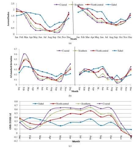
Figure 2. (a) Monthly cycle of mean Aerosol Index from TOMS (left) and OMI (right) (b) Monthly cycle of TOMS (left)
and OMI (right) AI standard deviation (c) differences between OMI and TOMS.
month, season and zone of maxima and minima. Furthermore, TOMS provides lower AI values compared with the OMI high values (Figure 2), possibly due to OMI’s greater spatial resolution and greater sensitivity to AI detection [14]. These variations are systematic as presented in Figure 2(c). From April to October, the pattern of the increase is similar across the four zones. Furthermore, the differences in AI between TOMS and OMI are larger between April to October especially in the North central southern and coastal zones. Finally, the differ-ences increase from the coastal zone towards the Sahel. However, in December, February and March, the dis-crepancies are higher in the Sahel and decrease towards the coastal zone. The systematic pattern in the variations of the values of AI measured by the two satellites can be related to the large variation in the meteorological con-ditions of the study regions.
(TOMS) and 0.047, 0.085, 0.103 and 0.110 (OMI) for the four zones of Nigeria. It is observed that these uncer-tainties from both sensors depend on latitude which is larger in TOMS. These results are consistent with the conclusion of Christopher et al.[24] and the observation in Figure 2(c) which revealed the pattern of the differ-ences. The standard errors were also estimated for Harmattan and summer which generally revealed higher val-ues larger for OMI (0.078, 0.100, 0.088 and 0.075) compared to TOMS (0.055, 0.074, 0.076 and 0.080 (TOMS). However, the uncertainty decreases and are generally larger 0.029, 0.043, 0.040 and 0.019 for TOMS and smaller for OMI 0.028, 0.036, 0.036 and 0.017 during summer period.
These consistencies allow the conclusion that the monthly mean AI has a distinct annual cycle in each zone, with the lowest values during the summer season (April-October) and the highest values during the Harmattan season (Nov-Mar). The increase in AI usually starts between August and September, when the aerosol concen-tration begins to build up. These aerosols are mainly UV-absorbing aerosols [14], because only positive AI val-ues are observed over Nigeria. The AI increases from September to January at different rates and generally reaches its peak in January in the north-central, southern, and coastal zones. This can be related to their close re-lations in climatic conditions, especially between the southern and coastal zones. However, in the Sahel, the AI fluctuation presents a unique pattern, increasing from August and reaching its maximum (peak) in March. As the rainfall in the summer begins in February in the south and April in the extreme north, gradual decreases in AI values are observed in the respective zones. However, a moderate concentration of UV-absorbing aerosols (AI > 0.5) is observed during April, indicating that there is still evidence of suspended particles in the atmosphere. In the southern and coastal zones, the AI decreases at a faster rate between February and May and at a slower rate from May to October. In the north-central, the AI decreases faster between March and May and slower between May and June than between July and October. However, in the Sahel zone, the AI decreases at a faster rate be-tween June and August. When the AI increases/decreases at a faster rate, usually the corresponding percent in-crease or dein-crease becomes larger, indicating that a large amount of aerosol is added due to frequent dust activi-ties or removed due to frequent rainfall. The lowest AI is observed around August in the Sahel and north central, while it is in September in the southern and coastal zones because of the extreme and intense rainfall. These patterns of monthly cycles (increasing) from August to March in the Sahel and September to January in the oth-er three zones as well as the decrease during the summoth-er remain consistent ovoth-er the 30 years of study, indicating that Nigeria usually experiences an increased concentration of absorbing aerosols during these months.
It is also observed from Figure 2(a) that from December to February, the AI is generally higher in the South-ern zone compared to the northSouth-ern zone. On the other hand, the AI is higher in the northSouth-ern zones compared to the southern from April to November. These monthly variations of the AI in Nigeria are related to the monthly variations in the meteorological conditions. The mean monthly OMI AIs presented are compared with those ob-served by Salman et al.[16] over Pakistan and Koskoutis et al.[14] over Greece, and the significant differences observed can be related to differeces in the climatic conditions and geo-location.
The observed cyclic variability of AI is mainly due to the seasonal cycle of elevated dust and smoke particles and the reduction in aerosol concentration by wet deposition [3]. An almost similar conclusion was made by Nwafor et al.[25] using Aeronet data at the Ilorin station (Southern zone of Nigeria), that the majority of the aerosol species in Ilorin originate from continental desert dust and biomass burning. They found that the contri-butions from industry and traffic emissions are insignificant in the total aerosol loading in the atmosphere over Ilorin. The seasonal cycle of dust transport has been noted by Goudie et al.[26]. The authors have showed that Saharan dust is regularly transported by strong winds from its source along its main path towards West Africa. This transport takes place from October to April of every year. During this period, the dust is transported at high altitudes [27] over a long distance towards Atlantic Ocean, which is believed to be the key factor responsible for the high AI in Nigeria. In addition to seasonal dust transport, local anthropogenic emissions in preparation for the upcoming rainy season farming and biomass burning during Harmattan [19] also contribute to the high AI values over the whole country. Due to this strong seasonality of dust aerosols in Nigeria, the yearly cyclic varia-tions of TOMS and OMI AI are found to be similar to the cycle of AOD for Ilorin reported in Balarabe et al. [19]. We observed a significant variation in the OMI AI cycle compared to the OMI AI cycle observed by
Sal-man et al.[16] over Pakistan. The authors documented that the AI increases from January to May, remains
al-most constant until July and then gradually decreases to December over their study area.
0 1 2 3
Sahel N/Central Southern Coastal
TO
M
S A
I
Study Zones
(a)
0 0.5 1 1.5 2 2.5 3 3.5
Sahel N/Central Southern Coastal
O
MI
A
I
Study zones
(b)
Figure 3. Box-and-whisker plots of AI (a: TOMS, b: OMI) for the period from 1984-2000 and 2004-2013.
at the median value, while the whisker denote the maximum and minimum AI. The statistics are based on the monthly mean values. The variation in the AI range is statically significant at 95% confidence level. These vari-ations occur because the highest AI values are observed over the Sahel during the summer period and over the southern zones during Harmattan.
3.2. Spatial Distribution of AI
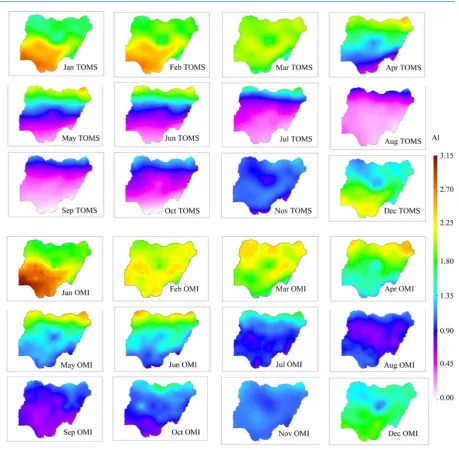
The results of the spatial distribution of AI are displayed in Figure 4. The figures show that the pattern of the monthly distribution of absorbing aerosols and hence atmospheric dust loading over Nigeria is not constant. Ra-ther, it exhibits a strong seasonality [28] in terms of loading along a north to south gradient. The AI distribution does not show a longitudinal zonation, as a result of which the longitude variations were maintained to reveal the stronger latitudinal changes. It is observed that at the beginning of the Harmattan period (November), the southern and coastal regions experienced an AI comparatively lower (below 1), except for areas around latitude 5.5˚N, than the north central and Sahel regions AI (~1). By December, the AI becomes close to 2 at multiple lo-cations in the south while only slightly above 1 in the Sahel and north central. This is due to the unstable at-mosphere in the south, which causes the aerosol layers to be uplifted at the upper level of the atat-mosphere, re-sulting in a high AI. However, in the northern zone, the stable atmosphere traps the aerosol layers at a lower height, resulting in a low AI.
From January to February, an extremely high AI (>2) was observed in the southern and coastal zones, except in the areas of Calabar, Uyo, Lagos, Warri and Onisha. On the other hand, these extreme values (AI above 2) occurred only at a few locations around Abuja and Yola in the north central and Sahel zones. It is observed that the AI becomes more intense throughout Nigeria between November and February (Harmattan), ranging from 0.87 - 2.07, 0.78 - 2.25, 0.64 - 2.63, and 0.62 - 2.64 (TOMS) and 0.95 - 2.40, 0.88 - 2.59, 0.88 - 2.90, and 0.83 - 2.92 (OMI) for the four zones. These AI values are indications of high levels of aerosol (dust and smoke) load-ing across the zones.
[image:9.595.164.459.83.312.2]Figure 4. Distribution of monthly mean AI, Jan-December, for TOMS (upper 3 rows) and OMI (lower 3 rows).
have been recognized as portions of the mountainous topography of Nigeria [28], which is characterized by a very high wind speed.
It is therefore obvious that the aerosol concentrations are higher in the south compared to the north from De-cember to February, while in the remaining months (March-November), the AI values are higher in the north, which is characterized by its proximity to the Sahara desert [3]. Regional anthropogenic activities are also re-sponsible for the AI variability and distribution [2]. Northern Nigeria is predominantly agricultural land, and ci-ties are usually semi-urban with large populations [30], where cooking involves the use of firewood and crop re-sidue. During the Harmattan months, the weather is extremely cold, requiring the continuous combustion of wood, animal dung and other fuels, which contributes to the increased absorption of aerosol [4]. The southern part of Nigeria is an industrially developed region, where local industries and other manmade emissions also contribute to the aerosol concentrations.
3.3. Distribution of Wind Speed, Visibility, Air Temperature and Relative Humidity
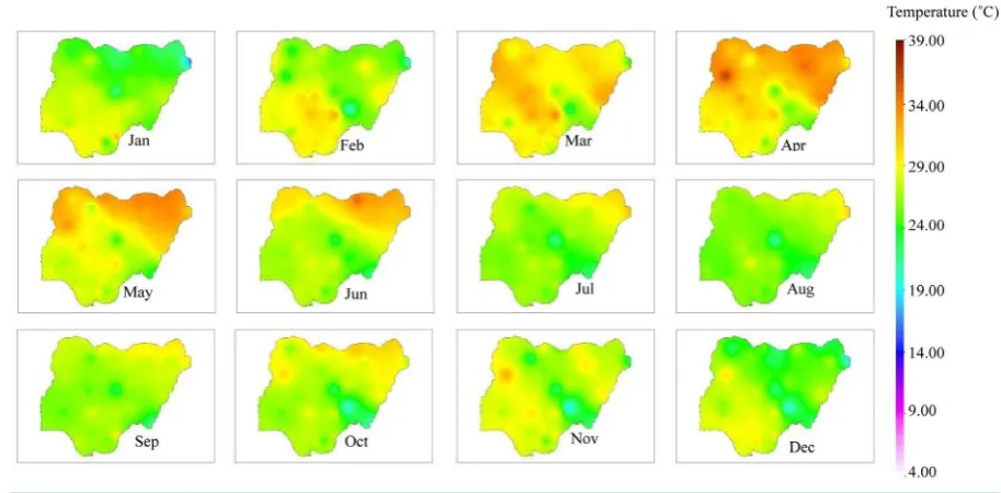
The variability of the AI in Nigeria can also be related to meteorological conditions. It is established that in all the seasons (throughout the year), the rainfall frequency and intensity are higher in the southern and coastal zones compared to in the north central and Sahel zones [31][32]. A similar pattern was observed for the relative humidity (Figure 5), and an opposite pattern for the wind speed (Figure 6). However, the visibility and temper-ature variations depend on the season, being high in the north during the summer and low in the south, with the opposite case during Harmattan (Figure 7 and Figure 8). These four meteorological parameters have a distinct annual cycle. For instance, the rainfall [32], high relative humidity (Figure 5), and good visibility (Figure 7) begin in April and increase along the latitude until they reach their respective peak periods. The peak period for the relative humidity is from July to September, that of visibility is May/June, and the rainfall peak varies be-tween June/July (in the southern and coastal regions) and August (in the north central and Sahel) [32]. For tem-perature (Figure 8), the highest values are observed from March to June, after which it shows an almost con-stant variation from June to September, except in the Sahel, where it was highest in June. The temperature is still significantly high in all zones from September to November. Therefore, the seasonal cycles of these parameters influence those of the AI variability within these months (March-September). For instance, the regions and sea-sons of frequent and intense rainfall as well as high relative humidity correspond to the regions of low AI values (Figure 2 and Figure 4) throughout Nigeria, leading to clear atmospheric conditions (good visibility). Signifi-cant AI values are observed in the north during the summer, which corresponds to the period of high tempera-ture and wind speed. This is because during the summer period, these parameters play a significant role for at-mospheric instability in the region, which in addition to the closeness to the source region, results in significantFigure 6. Distribution of monthly mean wind speed (January-December) between 1984 and 2013.
Figure 7. Distribution of monthly mean visibility (January-December) between 1984 and 2013.
AI concentrations. The highest AI concentration is also found to correspond to a period of high temperature (December to February) in the southern and coastal zones.
[image:12.595.86.542.200.560.2]Figure 8. Distribution of monthly mean temperature (January-December) between 1984 and 2013.
values are distributed over the entire region from one month to another. This can also be supported by Kaskoutis
et al.[1], who believes that the aerosol emissions, residence time, and diffusion ability depend mainly on wind
speed. During Harmattan, the high wind speed in the northern zones could be responsible for removing most of the incoming larger particles from the source region at the fastest rate, reducing the AI concentration. It can also be favorable for aerosol emissions at the local scale, resulting in a generally high AI in each zone compared to in the summer. On the contrary, the southern region is characterized by a low wind speed (Figure 6), which may enhance the aerosol residence time in the atmosphere, eventually leading to a high AI. Therefore, the monthly variations of the AI in Nigeria can be well justified by taking into account the corresponding monthly variations and distributions of meteorological conditions.
There are some blobs observed in Figures 5-8 which is more obvious in Figure 6 (wind speed) where me-teorological values denote very high values. This can be related to the occurrence of few observations in the af-fected parameter over a long period of time. These when average result to a significantly high values. Even though the higher values in wind speed is consistence with the available literature (28) revealing the regions of high wind speed in Nigeria.
3.4. Examination of Predicted AI Values
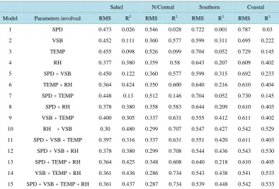
Table 1. Criteria used for selecting the new model for AI prediction.
Model Equation
1 AI = ao + a1(SPD)
2 AI = ao + a1(VSB)
3 AI = ao + a1(TEMP)
4 AI = ao + a1(RH)
5 AI = ao + a1(SPD) + a2(VSB)
6 AI = ao + a1(TEMP) + a2(RH)
7 AI = ao + a1(SPD) + a2(TEMP)
8 AI = ao + a1(SPD) + a2(RH)
9 AI = ao + a1(VSB) + a2(TEMP)
10 AI = ao + a1(VSB) + a2(RH)
11 AI = ao + a1(SPD) + a2(VSB) + a3(TEMP)
12 AI = ao + a1(SPD) + a2(VSB) + a3(RH)
13 AI = ao + a1(SPD) + a2(TEMP) + a3(RH)
14 AI = ao + a1(VSB) + a2(TEMP) + a3(RH)
15 AI = ao + a1(SPD) + a2(VSB) + a3(TEMP) + a4(RH)
Table 2. Result of the test of the overall model for generating the best subset.
Sahel N/Central Southern Coastal
Model Parameters involved RMS R2 RMS R2 RMS R2 RMS R2
1 SPD 0.473 0.026 0.546 0.028 0.722 0.001 0.787 0.03
2 VSB 0.452 0.111 0.360 0.577 0.599 0.311 0.695 0.222
3 TEMP 0.455 0.098 0.526 0.099 0.704 0.052 0.729 0.145
4 RH 0.377 0.380 0.359 0.58 0.643 0.207 0.609 0.402
5 SPD + VSB 0.450 0.122 0.360 0.577 0.599 0.315 0.692 0.233
6 TEMP + RH 0.364 0.424 0.350 0.600 0.640 0.216 0.610 0.404
7 SPD + TEMP 0.448 0.13 0.512 0.146 0.704 0.052 0.730 0.145
8 SPD + RH 0.378 0.380 0.358 0.583 0.644 0.209 0.610 0.403
9 VSB + TEMP 0.400 0.305 0.337 0.631 0.555 0.412 0.611 0.402
10 RH + VSB 0.30 0.480 0.299 0.707 0.547 0.427 0.542 0.529
11 SPD + VSB + TEMP 0.397 0.316 0.337 0.631 0.551 0.420 0.611 0.403
12 SPD + VSB + RH 0.378 0.380 0.299 0.708 0.544 0.436 0.543 0.530
13 SPD + TEMP + RH 0.364 0.425 0.348 0.608 0.640 0.218 0.610 0.405
14 VSB + TEMP + RH 0.361 0.436 0.286 0.734 0.543 0.438 0.541 0.533
15 SPD + VSB + TEMP + RH 0.361 0.437 0.287 0.734 0.539 0.448 0.542 0.533
RMSE when the two parameters are used. Therefore, model 10 (Equation 3) is chosen as the best model in each month and zone throughout this study.
[image:14.595.117.512.379.646.2]multicollinear-ity among the residuals usually leads to a great difficulty in separating out the individual effects of the variables involved. This was checked using the variance inflation factor (VIF). To check for bias due to multicollinearity, the approach by Marquardt [33] was used. The author believes that multicollinearity exists when the VIF is above 5 and becomes a problem when it exceeds 10; it was found to be between 1 and 3 in our analysis. The ef-fect of autocorrelations in a statistical model may be to overestimate R2 and underestimate the variance, which can also lead to a misleading conclusion. These were checked using the Durbin-Watson [34] test; in this regard, the author has established that values lower than 2 could be considered autocorrelation-free, as found in our analysis. Although a small departure from the normality assumption does not affect the model greatly, the F sta-tistics, confidence and prediction interval depend on the normality assumption. Therefore, we found it necessary to verify this assumption using a probability plot. The presence of heteroscedasticity biases the estimation of the standard error, which could also make drawing conclusions difficult. Finally, the potential outliers were re-moved based on Mahalanobis [35] and the Cook’s distance [36]. After removing the outliers, the remaining data points were divided into two sets for calibration and validation.
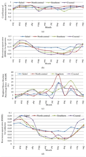
We hypothesize that the accuracy of the proposed AI prediction model for different months and zones should also depend on i) the distribution pattern of the measured AI values and the meteorological variables used as in-puts, ii) the season, because of the change in the altitude of the dust layer and weather conditions, and iii) the re-gion/zone. The performance of the model for each month was tested (Figures 9(a)-(d). The figures revealed the coefficient of determination (R2) for the calibration (Rr2), the root mean square error (RMSE) for calibration, weighted mean average percentage errors and the root mean square error (RMSE) for validation. The sensitivity of the AI prediction is low when the majority of the measured AI values is low and occurs within a smaller range of values. A similar situation was previously observed in developing an AOD prediction model during clear atmospheric conditions [20] [37]. For instance, most of the summer months (when AI is generally low) (Figure 9(a)) exhibited low R2, even though the corresponding root mean square errors (RMSE) are low (Figure 9(b)). For the Harmattan months (when AI is high with a large range of values), the accuracy (R2) of the prediction model improves, even though RMSE is large. However, during the transition period between Har-mattan and summer (April and October), the R2 values were significantly higher and the RMSE values were lower. Prediction models were also found to be more sensitive in the south and coastal areas during Harmattan due to the higher AI values, while the reverse is the case during the summer months. During the summer, R2 is generally higher in the Sahel and north central.
In general, the higher R2 values suggest that the meteorological variables used in the models explain a greater percentage of the AI variability in Nigerian zones. It also shows that the accuracy of the AI prediction improves when the aerosol concentration is high, which is in agreement with the above stated hypothesis.
The highest R2 is observed mostly during the period of November-April in all the zones except in Sahel where a significantly high R2 appears in July when the presence of dust in the atmosphere is still significant (AI > 1.5). These are months when the wind speed is generally high, the visibility is low and the relative humidity is also low (Figures 5-8). The R2 values range between 0.591 - 0.780, 0.641 - 0.809, 0.506 - 0.80, and 0.51 - 0.835 for the Sahel, north central, southern and coastal zones, respectively. These show how the meteorological variables can adequately explain the AI variability.
Given the criteria that a low wMAPE (Figure 9(c)) correspond to with a good prediction, the low value of wMAPE corresponding to relatively high R2 during Harmattan further explain the sensitivity of these models during Harmattan compared to summer period. It is also observed that during summer wMAPE was lowest in Sahel compared to other zones which clearly explain that during summer, models are more sensitive to AI pre-diction in Sahel than the other zones.
3.5. Validation of the Predicted AI
Here, we present the procedure to validate the proposed AI prediction model. To validate the model accuracy, the set of calibrated coefficients [a1 and a2] for each month and zone was used to generate a set of predicted AI values for the data set (J1, Jn) N. These predicted AI values were directly compared with the corresponding
0 0.2 0.4 0.6 0.8 1 Ja n Fe b Ma r Ap r Ma y Ju
n Jul Aug
Se p Oc t No v De c C o e ff ic ie n t o f d e te rm in a ti o n ( R 2) Month
Sa hel North centra l Southern Coa sta l
(a) 0 0.05 0.1 0.15 0.2 0.25 0.3 Ja
n Feb
Ma r Ap r Ma y Ju
n Jul
Au g Se p Oc t No v De c R o o t m e a n s q u a re e rr o r (R M S E ) fo r re g re ss io n Month
Sa hel North centra l Southern Coa sta l
(b) 0 5 10 15 20 25 30 35 40 Ja
n Feb
Ma r Ap r Ma y Ju
n Jul
Au g Se p Oc t No v De c W e ig h te d M e a n A b so lu te P e rc e n ta g e E rro
r w
M A P E (% ) Month
Sa hel North centra l Southern Coa sta l
(c) 0 0.01 0.02 0.03 0.04 0.05 0.06 0.07 0.08 0.09 0.1 Ja
n Feb
Ma r Ap r Ma y Ju
n Jul Aug
Se
p Oct
No v De c R o o t m ea n s q u a re e rro r (R M S E ) fo r v a lid a ti o n Month
Sahel North central Southern Coastal
(d)
Figure 9. Monthly distribution of (a) Coefficient of determination ( 2
r
R ); (b) Root mean square error of the regression; (c) The weighted mean percentage
error (wMAPE); (d) Root mean square error of the validation.
[image:16.595.167.459.83.615.2]0 0.5 1 1.5 2 2.5
Jan Fe
b r Ma Apr y Ma Jun lJu Aug Sep Oct Nov Dec
Pr
ed
ict
ed
A
er
os
ol
In
de
x
Month
[image:17.595.156.466.84.227.2]Sahel North central Southern Coastal
Figure 10. Monthly cycle of predicted Aerosol Index from TOMS.
calibrated RMSE and validated RMSE are related to the fact that there were under and over-predicted AI values owing to the non-uniform distribution of the aerosol in the atmospheric column. This may cause high deviations in our results, according to [20]
3.6. Comparison with Other Regression Models
We tried to compare the proposed model with other AI prediction models from the literature. The AI values pre-dicted by our model have already been compared to the measured AI values in the data for subset 2 in section 3.5. Anuforom et al.[3], Kehinde et al.[6] and Balarabe et al.[19] proposed a simple linear regression that re-lates the AI to the visibility data. It is important to know that the linear regressions by Anuforom et al.[3] and Kehinde et al.[6] were based on daily observations, including the retrieved missing TOMS AI data of 2001- 2003. It is also observed that the study by Anuforom et al.[3] is limited to the Sahel zone of Nigeria, while Ke-hinde et al.[6] provide linear regression models for eight individual stations in Nigeria. These actually limit our effort to make a detailed comparison with the exiting monthly models. However, their proposed simple linear regression models that relate the AI to the visibility data correspond to the proposed model number 2 in this work. From the Table 2, comparing the accuracy of this form of simple linear regression model proposed by the authors to the proposed model 10, it is clear that the proposed MLR model produced high R2 and lower RMSE. Kaskoutis et al.[14] and Salman et al.[16] suggested a similar monthly linear regression model for the AI pre-diction using precipitation as an input parameter. It important to note that rainfall is not considered part of the input parameters in this model, largely due to the long dry season in Nigeria, particularly in the Sahel and North central zones. However, their models yielded very low R2 values, much lower than those in our models for each month and zone.
4. Conclusions
In this study, the AI deduced from the TOMS and OMI over Nigeria from 1984 to 2013 is obtained. This is in view of analyzing its temporal and spatial variability in comparison with the available ground observations of wind speed, visibility, temperature and relative humidity in Nigeria. A new empirical (multiple regression) model that allows an estimation of the values of AI in Nigeria based on these data is developed. The results show that the monthly mean AI has a distinct annual cycle in each zone, with lowest values during the summer season (April-October) and the highest values during the Harmattan seasons (Nov-Mar). This shows continuity in the seasonal pattern of dust aerosol emission, transport, and removal over the 30-year period under study. It also exhibits a strong north to the south gradient in terms of loading. The months of the maximum correspond to dry weather responsible for dust emission and transport, while the minima correspond to the wet/rainy period, when aerosols are removed from the atmosphere.
and 2001- 2003. This model is the first empirical correlation model to use in-situ meteorological observations to predict AI. Due to the absence of these types of models in the available literature, a comparison of its accuracy with that of existing models is difficult. The model was used to calculate the monthly AI for those missing years and the values were compared with the measured AI. It is found that the temporal characteristics of the predicted (missing) AI are similar to those of the measured AI. The model validation RMSE shows very high correlation with the regression RMSE, which implies a strong relationship between the predicted and measured AIs. How-ever, under-estimation is observed in the AI retrieval, which resulted in the differences between the calibrated RMSE and validated RMSE. These are related to the non-uniform distribution of the aerosols in the atmospheric column.
The accuracy of the proposed AI prediction model for different months and zones was found to be related to i) the distribution pattern of the measured AI values, as well as the meteorological variables used as inputs; ii) the season, because of the change in the altitude of the dust layer and weather conditions; and iii) the region/zone. The AI is higher during the dry months (Harmattan season) and lower during the wet months (rainy/wet season) in all zones. It is recommended that an empirical model for AI prediction on the basis of frequent cloud forma-tion on a daily basis that accounts for all meteorological variaforma-tions be produced.
Acknowledgements
The authors gratefully acknowledge the financial support by ESCAP-NASDA (grant no. 304/PFIZIK/650049/ E012). The visibility and meteorology data were provided by the NOAA/NESDIS/NCDC, the authors, for this reason, wish to thank Stuart Hinson a Meteorologist, NOAA-NCDC for providing the data. They also wish to thanks, TOMS and OMI AI processing team. Finally we acknowledge Dr. Tan Fuyi, for the time he devoted at various discussions regarding this work.
References
[1] Kaskaoutis, D.G., Kambezidis, H.D., Nastos, P.T. and Kosmopoulos, P.G. (2008) Study on an Intense Dust Storm over Greece. Atmospheric Environment, 42, 6884-6896. http://dx.doi.org/10.1016/j.atmosenv.2008.05.017
[2] N’Tchayi, M.G., Bertrand, J.J. and Nicholson, S.E. (1997) The Diurnal and Seasonal Cycles of Desert Dust over Africa North of the Equator. JournalofAppliedMeteorology, 36, 868-882.
http://dx.doi.org/10.1175/1520-0450(1997)036<0868:TDASCO>2.0.CO;2
[3] Anuforom, A.C., Akeh, L.E., Okeke, P.N. and Opara, F.E. (2006) Inter-Annual Variability and Long-Term Trend of UV-ab-Sorbing Aerosols during Harmattan Season in Sub-Saharan West Africa. Atmospheric Environment, 41, 1550- 1559. http://dx.doi.org/10.1016/j.atmosenv.2006.08.024
[4] Prospero, J.M., Ginoux, P., Torres, O., Nicholson, S.E. and Gill, T.E. (2002) Environmental Characterization of Global Sources of Atmospheric Soil Dust Identified with the Nimbus-7 Total Ozone Mapping Spectrometer (TOMS) Absorb-ing Aerosol Product. ReviewsofGeophysics, 40, 2-1-2-31. http://dx.doi.org/10.1029/2000RG000095
[5] NFNC (Nigerian’s First National Communication) (2003) Under the United Nation Frame Work Convention on Cli-mate Change. Federal Republic of Nigeria, 1-132.
[6] Kehinde, O.O., Ayodeji, O. and Vincent, O.A. (2012) A Long-Term Record of Aerosol Index from TOMS Observa-tions and Horizontal Visibility in Sub-Saharan West Africa. International Journal of Remote Sensing, 33, 6076-6093. http://dx.doi.org/10.1080/01431161.2012.676689
[7] Momadou, S.D., Moctar, C. and Amadou, T.G. (2013) Intra-Seasonal Variability of Aerosol and Their Radiative Im-pacts on Sahel Climate during the Period 2000-2010 Using Aeronet Data. International Journal of Geosciences, 4, 267-273. http://dx.doi.org/10.4236/ijg.2013.41A024
[8] Wei, H.J., Tan, H.K., Weimin, S., Guixiang, S., Guohai, C., Lili, J., Cheng, J., Renjie, C. and Bingheng, C. (2009) Vi-sibility, Air Quality and Daily Mortality in Shanghai China.Science of the Total Environment, 407, 3295-3300. http://dx.doi.org/10.1016/j.scitotenv.2009.02.019
[9] Habib, G., Venkataraman, C., Chiapello, I., Ramachandran, S., Boucher, O. and Reddy, M.S. (2006) Seasonal and Inte rannual Variability in Absorbing Aerosols over India Derived from TOMS: Relationship to Regional Meteorology and Emissions. AtmosphericEnvironment, 40, 1909-1921. http://dx.doi.org/10.1016/j.atmosenv.2005.07.077
[10] Singh, A. and Sagnik, D. (2012) Influence of Aerosol Composition on Visibility in Megacity Delhi. Atmospheric En-vironment, 62, 367-373. http://dx.doi.org/10.1016/j.atmosenv.2012.08.048
At-mospheric and Solar-TerrestrialPhysics, 84, 75-87. http://dx.doi.org/10.1016/j.jastp.2012.05.014
[12] Kalu, A.E. (1979) The African Dust Plume: Its Characteristics and Propagation across West Africa in Winter. In: Mo-rale, C., Ed., Saharan Dust Mobilization, Transport, Deposition, Wiley, New York, 95-118.
[13] Omotosho, J. (1989) Equivalent Potential Temperature and Dust Haze Forecasting at Kano, Nigeria. Atmospheric Re-search, 23, 163-178. http://dx.doi.org/10.1016/0169-8095(89)90005-7
[14] Kaskaoutis, D.G., Nastos, P.T., Kosmopoulos, P.G. and Kambezidis, H.D. (2010) The Aura-OMI Aerosol Index Distri bution over Greece. AtmosphericResearch, 98, 28-39. http://dx.doi.org/10.1016/j.atmosres.2010.03.018
[15] Chiapello, I., Prospero, J.M., Herman, J.R. and Hsu, N.C. (1999) Detection of Mineral Dust over the North Atlantic Ocean and Africa with the Nimbus 7 TOMS. Journal of Geophysical Research, 104, 9277-9291.
http://dx.doi.org/10.1029/1998JD200083
[16] Salman, T. and Muhammad, A. (2015) Spatio-Temporal Distribution of Absorbing Aerosols over Pakistan Retrieved from OMI Onboard Aura Satellite. Atmospheric Pollution Research, 6, 1-12.
[17] Israelevich, P.L., Levin, Z., Joseph, H. and Ganor, E. (2002) Desert Aerosol Transport in the Mediterranean Region as Inferred from the TOMS Aerosol Index. Journal of Geophysical Research, 107, 4572.
http://dx.doi.org/10.1029/2001jd002011
[18] Kiss, P., Jánosi, M.I. and Torres, O. (2007) Early Calibration Problems Detected in TOMS Earth-Probe Aerosol Signal.
Geophysical Research Letters, 34, Article ID: L07803. http://dx.doi.org/10.1029/2006GL028108
[19] Balarabe, M., Abdullah, K. and Nawawi, M. (2015) Long-Term Trend and Seasonal Variability of Horizontal Visibili-ty in Nigerian Troposphere. Atmosphere, 6, 1462-1486. http://dx.doi.org/10.3390/atmos6101462
[20] Tan, F., Lim, H.S., Abdullah, K., Yoon, T.L. and Holben, B. (2015) Monsoonal Variation in Aerosol Optical Properties and Estimation of Aerosol Optical Depth Using Ground-Based Meteorological and Air Quality Data in Peninsular Ma-laysia. Atmospheric Chemistry and Physics, 15, 3755-3771. http://dx.doi.org/10.5194/acp-15-3755-2015
[21] Papadimas, C.D., Hatzianastassiou, N., Mihalopoulos, N., Querol, X. and Vardavas, I. (2008) Spatial and Temporal Variability of Aerosol Properties over Mediterranean Basin Based on 6 Years (2000-2006) MODIS Data. Journal of Geophysical Research, 113, Article ID: D11205. http://dx.doi.org/10.1029/2007jd009189
[22] Herman, J.R., Bhartia, P.K., Torres, O., Hsu, C., Seftor, C. and Celarier, E. (1997) Global Distribution of UV- Absorbing Aerosols from Nimbus 7/TOMS Data. JournalofGeophysicalResearch Atmospheres, 102, 16911-16922. http://dx.doi.org/10.1029/96JD03680
[23] Torres, O., Bhartia, P.K., Herman, J.R., Ahmad, Z. and Gleason, J. (1998) Derivation of Aerosol Properties from Satel-lite Measurements of Backscattered Ultraviolet Radiation. Theoretical Basis. Journal of Geophysical Research Atmos-pheres, 103, 17099-17110. http://dx.doi.org/10.1029/98JD00900
[24] Noori, R., Hoshyaripour, G., Ashrafi, K. and Araabi, B.N. (2010) Uncertainty Analysis of Developed ANN and ANFIS Models in Prediction of Carbon Monoxide Daily Concentration. Atmospheric Environment, 44, 476-482.
http://dx.doi.org/10.1016/j.atmosenv.2009.11.005
[25] Christopher, S.A., Gupta, P., Haywood, J. and Greed, G. (2008) Aerosol Optical Thicknesses over North Africa: 1. Development of a Product for Model Validation Using Ozone Monitoring Instrument, Multiangle Imaging Spectro Ra-diometer, and Aerosol Robotic Network. Journal of Geophysical Research, 113, Article ID: D00C04.
http://dx.doi.org/10.1029/2007JD009446
[26] Nwafor, J.C. (2007) Global Climate Change, the Driver of Multiple Causes of Flood Intensity in Sub-Saharan Africa.
The International Conference of Climate Change and Economic Sustainability, Nnamdi Azikiwe University, Awka, 25 July 2007, 12-14.
[27] Goudie, A.S. and Middleton, N.J. (2001) Saharan Dust Storms: Nature and Consequences. Earth-Science Reviews, 56, 179-204. http://dx.doi.org/10.1016/S0012-8252(01)00067-8
[28] Wolfgang, S. and Brigitta, S. (2008) Meteorological Causes of Harmattan Dust in West Africa. Geomophology, 95, 412-428. http://dx.doi.org/10.1016/j.geomorph.2007.07.002
[29] Oyem, A.A. and Igbafe, A.F. (2010) Analysis of Atmospheric Aerosol Loading over Nigeria. EnvironmentalResearch Journal, 4, 145-156. http://dx.doi.org/10.3923/erj.2010.145.156
[30] Olugunorisa, T.E. and Tamuno, T.T.T. (2003) Spatial and Seasonal Variation of Sandstorm over Nigeria. Journalof TheoreticalandAppliedClimatology, 75, 55-63.
[31] Hopkins, M. (1991) Human Development Revisited: A New UNDP Report. World Development, 19, 1469-1473.
[32] Philip, G.O., Babatunde, J. and Gunnar, A.L. (2011) Rainfall Trends in Nigeria 1901-2000. JournalofHydrology, 411, 207-218. http://dx.doi.org/10.1016/j.jhydrol.2011.09.037
[33] Marquardt, D.W. (1970) Generalized Inverses, Ridge Regression, Biased Linear Estimation, and Nonlinear Estimation.
[34] Durbin, J. (1970) Testing for Serial Correlation in Least-Squares Regressions When Some of the Regressors Are Lagged Dependent Variables. Econometrica, 38, 410-421. http://dx.doi.org/10.2307/1909547
[35] Mahalanobis, P.C. (1936) On the Generalised Distance in Statistics. ProceedingsoftheNationalInstituteofSciences
of India, 2, 49-55.
[36] Sanford, R. and Cook, D.W. (1982) Residuals and Influence in Regression. Chapman & Hall, New York.
[37] Zhong, B., Liang, S. and Holben, B. (2007) Validating a New Algorithm for Estimating Aerosol Optical Depths over Land from MODIS Imagery. International Journal of Remote Sensing, 28, 4207-4214.
http://dx.doi.org/10.1080/01431160701468984