Constructing a GDP based Index for Use as Benchmark

Constructing a GDP-based Index for Use

as Benchmark

Cohen, Ruben D

October 2009

Constructing a

GDP

-based Index for Use as Benchmark

Ruben D. Cohen

Abstract

The gross domestic product [GDP] is a fundamental economic indicator that is frequently used as a benchmark for local equity indices. The widespread appeal of this association is understandable because an equity index, especially if broad, could, like the GDP, also manifest the state of the economy. At the same time, however, the validity of a direct relation between the two is debatable since the GDP is known to be characteristically different from the typical equity index, however broad.

In this work, we review some of the key elements that separate the GDP from a typical broad equity index in order to explain why the two cannot be compared directly with each other. We then incorporate a readily available mapping technique to create a

GDP-based index that circumvents their inherent disparities and, thus, enable us to benchmark one against the other.

Introduction

The GDP, in level or growth rate, is one of the most commonly used indicators that reflect the state of a country’s economy. There is no need to describe here how this

parameter is defined or estimated, as there is an extensive literature that covers it. What

is relevant to this work is that this measure, which is, in one form or another, used as a

benchmark for various local equity indices, begins first as a forecast over some time

horizon, which is soon followed by a revision. The closed-loop revising process

continues iteratively until the target date is reached, by which time convergence occurs.

At this stage, the GDP becomes realized and, thus, “historical” and the process repeats itself with a new prediction towards a new target date. The time span for this cycle, from

prediction to convergence, normally equals one quarter, which is the reporting time scale

for many economic indicators.

The drive to speculate on what the future holds for the GDP3, as well as many other economic indicators, is fuelled by a society’s need to invest and grow A correct

guess could guide one to the right investment decision, which would, in turn, lead to

1

Citi, London E14 5LB, UK.

2

I express these views as an individual, not as a representative of companies with which I am connected.

3

higher productivity, growth in real profits and, subsequently, personal wealth. This

speculative approach to linking the GDP with profits remains, in fact, essential to the development of any competitive economy that thrives on investment and growth. At the

other extreme, also, after the speculations have been revised over and over and the true

GDP number comes to light, it will, purely by construct, embody the profits that underlie its constituents.

The circular relationship that the GDP has with profits, as summarised above, is, therefore, one reason why the indicator is used regularly as a benchmark for “broad“4

equity indices [Faugère & Van Erlach (2006), Honnerová (2003), and many others].

Examples of such comparisons abound, whereby one simply has to open a financial

publication [newspaper, magazine, etc.] to find them.

Considering all this, however, there is still the issue that a direct relationship

between the two is not universally recognized (Kerschner et al_{, 1999). There are several}

reasons for this, among which are that (1) the GDP is based mainly on revenues, whereas equity valuation, the very basis of any equity index, centers on profits, (2) a typical

equity index has a higher exposure to foreign earnings than does the GDP, (3) the GDP

level, or index, is measured in units of income [i.e. $/year], whereas an equity index is

denominated in value [i.e. $] and last, but not least, (4) by the time the GDP converges from speculation to historical, which could take up to several months depending on the

forecast horizon, the number becomes actual. This contrasts sharply to what an equity

index symbolizes, which is merely a speculation on the underlying firms’ earnings

potential going forward.

On a macro level, one could, more or less, get around statements (1) and (2)

above, but not (3) and (4). In reference to (1), for instance, one could claim that a

company’s expenses comprise another company’s profits, so that a merger between the

two can create a conglomeration that generates only revenues. Thus, while taking the

two companies separately is akin to an equity index whose overall value is determinable

by individual profits, their merger becomes analogous to the GDP, which tracks revenues.

4

Similarly, one could argue against (2) in that just as companies compete against

each other economically, jurisdictions do so as well, but on a grander scale. For

example, while an equity index in Country A, with an exposure to Country B, would contribute to, or gain from, the GDP of Country B, an equity index in Country B, with an exposure to Country A, would contribute to, or gain from, Country A’s GDP. This closed cycle, therefore, would have a compensating effect on an equity index, enabling its

foreign exposure to circle back into the GDP and, subsequently, the local equity indices and vice versa. As result, one should, effectively, be able to compare, albeit not directly,

the characteristics of a country’s GDP to the local, broad indices.

Statements (3) and (4), on the other hand, hinge on deeper fundamental

discrepancies between the GDP level and an equity index and, thus, are more challenging to crack. Here, as a consequence, one must follow a different path when trying to

correlate the two parameters. Establishing this path and providing evidence for it, with

intent to develop a GDP-based index for benchmarking purposes, constitute the remainder of this paper.

Relating the GDP _{With an Equity Index}

There are, as mentioned above, two primary reasons5 why the GDP cannot serve directly as a benchmark for an equity index. Firstly, different units of measure characterize the

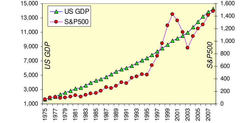
two parameters and, secondly, while the GDP reflects an actual, quantifiable number, the value of an equity index is entirely speculative. Proof for the latter can be observed in

Figure 1, where the historical level of the US nominal6 GDP is displayed alongside the

S&P5007 index, both plotted from 1975 to 2008. Here, although there is similarity in long-term trends, one could easily spot the difference in volatility between the two

quantities, where the higher volatility in the S&P500 is a manifestation of the speculations that shape it. In consequence, one must rely on an alternative way to

accomplish the task of benchmarking an equity index, a speculative-based measure,

5 _{As given by statements (3) and (4) in the previous section.} 6

Nominal instead of real because the equity index is in nominal terms.

7

against the GDP, which is a realized number, not to mention the other differences already listed above.

Figure 1 – Comparing the trends of the nominal US GDP level and S&P500 index between 1975 and 2008. The higher volatility in the latter is a manifestation of its underlying speculative nature.

1,000 3,000 5,000 7,000 9,000 11,000 13,000 15,000 19 75 19 77 19 79 19 81 19 83 19 85 19 87 19 89 19 91 19 93 19 95 19 97 19 99 20 01 20 03 20 05 20 07 0 200 400 600 800 1,000 1,200 1,400 1,600 US GDP S&P500 U S GD P S&P5 0 0

The alternative being considered here is founded on a readily existing

methodology that can be also used to assess the relative valuation between the nominal

level in GDP and an equity index. As a detailed derivation of the model is available elsewhere (Cohen, 2005), we shall avoid re-deriving it here and, instead, provide a brief

summary of the notions that underlie it and the final outcome itself.

Beginning with the supposition that the value of a publicly traded security at a

macro level [i.e. a broad equity index] depends on two parameters, one being the

nominal8 interest rate and the other time9, it can be shown that

(1)

) ( lnS−bt =Ψ b

where S is the level of the index, b is the interest rate, t is an annual10 measure of time and Ψ(b) is some function of b. There are several implications to the above relationship, more notably that Ψ turns out to be a function of only b. This means that a plot of Ψ

8

See Footnote 6.

9

Refer to Cohen (2005) for a justification of how the two parameters were selected.

10

against b within some time range t1 to t2 should, in the absence of any outliers and

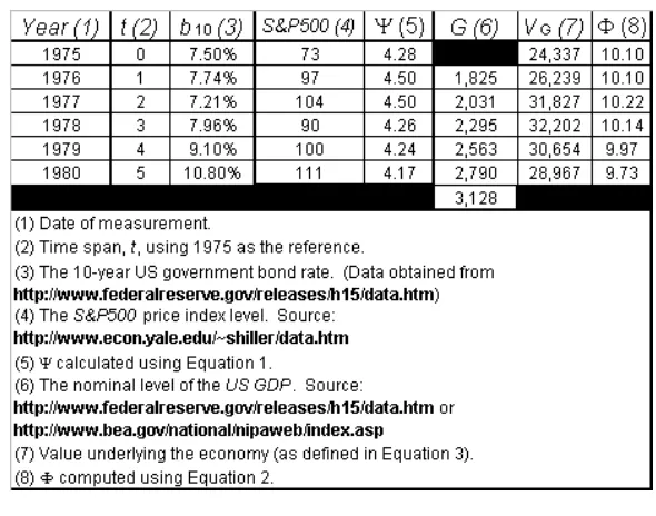
structural shifts in the economy, yield a single, continuous curve, depending only on b. Table 1 provides an example of how Ψ is calculated from Equation 1, given S and

b10 [b10 is the 10-year US government bond rate] at any time, t. In the case of 1977, for

instance, where t, b10 and S are 2, 7.21% and 104, respectively, Ψ becomes

. 50 . 4 2 % 71 . 7 ) 104

ln( − × = 11

Table 1 – An example calculation of the function Ψ in Column 5, given t, b and S in Columns 2-4, respectively. Columns 6-8, refer to the GDP, the treatment of which shall be discussed shortly.

The sample data in Table 1, starting with 1975, shows a time parameter, t, which begins at 0, thus defining 1975 as the “reference” date. In fact, it does not matter what

date is used as the reference, since the impact of this on the function Ψ is linear and

cancels out in subsequent calculations.

Table 1 contains three additional elements, all which are manifested in Columns

6-8 and pertain to the GDP. The parameter G in Column 6 is the nominal level of the US GDP in billions of dollars. The treatment of G, also described in detail in Cohen (2005), leads to the following relationship

(2)

) ( lnV_G −bt =Φ b

11

which is directly analogous to Equation 1. Here, however, VG, which replaces the index,

S, in Equation 1 represents the “value” of the economy at time t and is defined as follows:

) ( 1) ( ) ( t b t G t

V_G ≡ + (3)

where G(t+1) is the nominal GDP level one year ahead of t and b(t) is the interest rate at time t. Therefore, since G is defined by units of earnings - $/year – VG will then acquire

the units of value - $ - thus allowing direct association between Equations 1 and 3,

representing an equity index and the GDP’s implied value, respectively

The reason for the 1-year gap in measurement time between G and b in Equation 3 has to do with how asset valuation is generally conducted in practice, which is based on

forward looking earnings. In addition, if t represents today, t+1 would be one year from today, thus deeming G(t+1) a forecast and, hence, a speculation, just like an equity index [refer again to Cohen (2005) for a more detailed explanation].

An example of how Φ is calculated follows from the sample data in Table 1. In

reference to 1977, similar to the earlier illustrative calculation for Ψ, VG is computed as

leading, subsequently, to

. 827 , 31 % 21 . 7 / 295 , 2 ) t ( / ) 1

(t+ b = =

G 22 . 10 2 % 21 . 7 ) 22 . 10 ln( ln ) ( = − = − × =

Φ b V_G bt

Impact of Different Maturities

Although the interest rate, b, is a primary input to the model described above, its maturity has not been specified simply because it turns out to be irrelevant. What matters,

though, is that b must be represented by a government bond rate, since a government bond is typically free of any firm-specific risks [credit, liquidity, etc.].

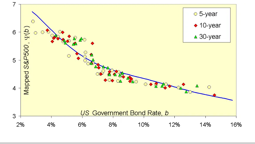
Figures 2a and 2b show Ψ and Φ, which relate to the S&P500 index and the US

Figure 2a – The function Ψ(b), defined by Equation 1 and based on the S&P500 index, is plotted here against b for different maturities. It illustrates, firstly, the irrelevance of the maturity of b

and, secondly, the convergence of the data around b.

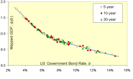
Figure 2b – The function Φ(b), defined by Equation 3, is plotted here against b for different maturities. Again, it depicts the irrelevance of the maturity of b, as well as the convergence of the data around b. The convergence is significantly tighter in this case than in Figure 2a, owing to the fact that the GDP is a realized number rather than speculated. The line is a best-fit polynomial

An important feature in Figures 2a and 2b is the convergence of both functions Ψ

and Φ around b, which is implicit in how Equations 1 and 3 are derived. Never the less, Φ's convergence is markedly tighter because the GDP is a realized number, whereas the equity index, which underlies Ψ in Figure 2a, is purely speculative. Another prominent

attribute, particularly in Figure 2b, is that the impact of the different rate maturities is

indeed irrelevant.12

Finally, for estimation purposes, the mapped GDP data in Figure 2b have been curve fitted with a polynomial of order 6, characterizing Φ as a function of b alone13. The single curve traverses all the different maturities considered, having taken into

account their irrelevance.

Defining the New GDP_{-based Benchmark}

With the above as background, we now proceed to construct the proposed GDP-based index for benchmarking purposes. For this, we refer to Figures 2a and 2b and note the

difference in the levels across Ψ and Φ, which is, exclusively, a result of the disparity in

the measurement scales between the GDP and the equity index, here being the S&P500. Subtracting a constant, αΦΨ, from the level of Φ, thus shifting it down in parallel to

coincide with Ψ, could easily circumvent this – i.e.:

ΦΨ

− Φ =

Ψ(b) (b) α (4)

which leads to

ΦΨ

− =ln _G α

lnS V (5)

12

More examples of this nature, related to different jurisdictions, can be found in Cohen (2005).

13

upon combining Equations 1, 2 and 4. Minimizing the sum of squared errors between the

data points in Figure 2a and the fitted curve in Figure 2b gives α_ΦΨ ≈5.41.

Figure 3 depicts the fit between the curve in Figure 2b, as it is lowered by a

constant value of 5.41 to the level of the data in Figure 2a. The comparison is

satisfactory, attesting to a more direct relationship between the S&P500 index and VG, as

presented in Equation 5.

Figure 3 – Lowering the best-fit curve in Figure 2b by a constant, αΦΨ, equal to 5.41 and

corresponding to the S&P500 index, and inserting into Figure 2a to compare with Ψ(b).

The constant, αΦΨ, will, of course, vary with other indices, depending on their

scales relative to VG. As an example, αΦΨ for the DJIA index turns out to be

approximately 3.30, whose fit with the same line in Figure 2b, but parallel shifted, is

portrayed in Figure 4. The strong similarity between Figures 3 and 4, relating to the

S&P500 and DJIA indices, respectively, is due to the high correlation between the two indices. As high correlation among broad equity indices is generally the norm, the newly

constructed GDP-based benchmark, corrected for αΦΨ, could thus have large-scale

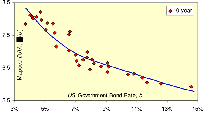
Figure 4 – Similar to Figure 3 and for the same time range, but for the DJIA index. The solid line is the best-fit line in Figure 2b, but with a parallel shift and an αΦΨ of about 3.30. To reduce the

clutter, the figure includes the function Ψ based on only b10.

5.5 6.5 7.5 8.5

3% 5% 7% 9% 11% 13% 15%

10-year

US _{Government Bond Rate,} b

M

a

pp

ed

DJ

IA

,

(

b

)

Next, upon exponentiating Equation 5, one can finally define S as a GDP-based benchmark for any broad equity index. In the case of S&P500, for instance,

incorporating 5.41 for αΦΨ leads to:

6 . 223 / )

exp( VG VG

S_S&P500 = −α_ΦΨ × = (6)

where SS&P500 represents the benchmark for the S&P500 index. Figures 5a-b compare the

S&P500 index against its GDP-based benchmark, SS&P500, both plotted against the year,

ranging from 1975 to 2008. Being linear in scale, Figure 5a amplifies the differences at

higher levels, whereas its logarithmic counterpart, Figure 5b, helps provide an objective

comparison over the entire range of the time scale.

Prior to continuing on, we observe that the benchmark in Figures 5a-b is based on

b10 only, knowing well that VG in Equation 6 depends on the maturity that one ultimately

chooses. The reason for focusing on a single rate, rather than all three considered here, is

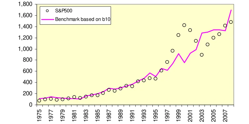
Figure 5a – Comparison of the new GDP benchmark, as calculated from Equation 6 and based on

b10, with the S&P500 index.

0 200 400 600 800 1,000 1,200 1,400 1,600 1,800 19 75 19 77 19 79 19 81 19 83 19 85 19 87 19 89 19 91 19 93 19 95 19 97 19 99 20 01 20 03 20 05 20 07 S&P500

Benchmark based on b10

Figure 5b – Same as Figure 4a, but in logarithmic scale. 10 100 1,000 10,000 19 75 19 77 19 79 19 81 19 83 19 85 19 87 19 89 19 91 19 93 19 95 19 97 19 99 20 01 20 03 20 05 20 07 S&P500

Benchmark based on b10

Figure 6, on the other hand, is included here as well to depict how the proposed

GDP benchmark might vary depending on the different interest rate maturities that could go into calculating VG. In this example, where the behavior of the benchmarks is

displayed based on the 5 and 10-year maturities, we observe that, although the long-term

trend is very similar in both cases, there appear to be gaps that separate them in certain

caused by larger spreads in the corresponding yield curves, bearing in mind that this is

perhaps an outcome of underlying economic uncertainties. In contrast, tighter gaps result

from more horizontal yield curves, which, as discussed in Cohen (2006), could manifest

periods of higher economic certainty. Therefore, as described here, the link between the

maturity-induced gaps in the benchmarks and the spreads in the underlying yield curves

could, potentially, explain how economic uncertainty is transmitted to equity markets.

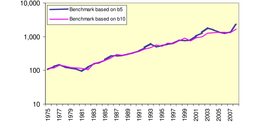
Figure 6 – Illustration of how the GDP-based benchmark, as given by Equation 6, differs depending on the maturity used to calculated VG. The gaps between the benchmarks reflect the spread in the

underlying yield curve, whereby larger spreads will lead to wider gaps and vice versa. 10 100 1,000 10,000 19 75 19 77 19 79 19 81 19 83 19 85 19 87 19 89 19 91 19 93 19 95 19 97 19 99 20 01 20 03 20 05 20 07

Benchmark based on b5

Benchmark based on b10

We finally refer back to Figures 5a-b and draw two important conclusions.

Firstly, the issue of different measurement units, as discussed earlier and depicted by the

use of two separate axes in Figure 1, is now resolved. The proposed method, effectively,

places both the equity index and its benchmark into the same category of units, thereby

allowing direct comparison between the two. Secondly, there is evidence of a better fit

between the S&P500 index and its benchmark in Figures 5a-b than that in Figure 1. In essence, the index in Figures 5a-b appears to follow its GDP-based benchmark more closely than it does the GDP alone. The gaps in Figures 5a-b are, in addition, observed to occur in times well known for their characteristic market slumps [i.e. mid 1970’s and

between 2001-2004] and bubbles [1997-2000]. Clearly, therefore, the benchmark is also

The appeal of the new benchmark goes beyond its satisfactory fit with the equity

index it allegedly portrays, or its ability to highlight periods of over/under valuation of

the index. Since the benchmark can be described in closed form, one should then also be

able to estimate its duration - an important property - more easily and objectively, as it

shall be demonstrated next.

Calculating the Duration of the New Benchmark

The duration of a financial instrument is normally defined as its sensitivity to the interest

rate, all else constant. There are certain issues with this generic definition, never the less,

which introduce a hurdle when it comes to practical implementation. These issues are two

fold and provoked mainly by the following questions: (1) sensitivity to what interest rate

in the yield curve and (2) how does one get around “all else constant”, which is critical to

the definition? Although these are non-issues when it comes to determining the duration

of a bond, owing to the existence of a close-form valuation relationship, they are major

when equities, equity indices and their related benchmarks are involved. This is likely due

to the lack of an objective and closed-form equity valuation relationship, as well as the

absence of some measure of maturity or investment horizon.

The literature, notwithstanding, does contain a number of works related to

computing the duration of equity. Here, for instance, there is the notion that a

combination of the book-to-market value and other ratios can provide a proxy for the

[implied] duration [Dechow et al _{(2004) and Santa-Clara (2004)]. In the case of equity}

portfolios and, likewise, indices, the use of the Dividend Discount Model [DDM] for estimating duration appears to dominate, although different authors have offered tweaked

versions of it. For example, while Casabona et al _{(1984) suggest directly implementing}

the DDM, Leibowitz et al _{(1989) propose incorporating a discount rate that takes into}

account an equity risk premium sensitive to both inflation and real rates. As related

works are abundant in the literature, it is perhaps better, in the interest of space, not to

delve deeply into them and, instead, proceed directly with obtaining the duration of the

new GDP-based benchmark introduced here.

(7)

ΦΨ − + Φ

= b bt α

S ( ) ln

where S denotes the benchmark, as defined earlier, and αΦΨ a constant. Now, based on definition, we write the following

t S

b S

D _⎟⎟

⎠ ⎞ ⎜⎜

⎝ ⎛

∂ ∂ −

≡ ln (8)

with DS representing duration, ∂lnS/∂t denoting sensitivity to the interest rate and the

subscript t symbolizing “all else constant.” Substituting 7 into 8 finally yields:

⎥⎦ ⎤ ⎢⎣

⎡ Φ ₊

−

= t

b b D

S _d

) ( d

(9)

Given the above, along with an estimate for Φ(b) based on the curve fit in Figure 2b [see polynomial in Footnote 13], one could, subsequently, compute the duration of the

benchmark, DS, without difficulty and in closed form. The choice of b - be it b5, b10, b30,

or any other that is preferred - is also easily implementable, owing to the irrelevance

property discussed earlier. How DS varies with the choice of b, therefore, would be

indicative of the benchmark’s sensitivity to the different maturities.

A sample calculation of the duration measure, as presented by Equation 9, is

Table 2 – Sample calculation of duration in accordance with Equation 9. 10-year rate has been selected here as the example.

The duration calculation in Table 2 has been extended to include the rates b5, b10

and b30, as well as taken through to 2008, with the outcome plotted in Figure 7. Here,

however, we have focused on 1990 onwards, so as to, once again, reduce clutter.

-5 0 5 10 15 20 25 30 35

2% 4% 6% 8% 10%

b5

b10

b30

D

u

ra

ti

o

n

, y

e

a

rs

Interest Rate

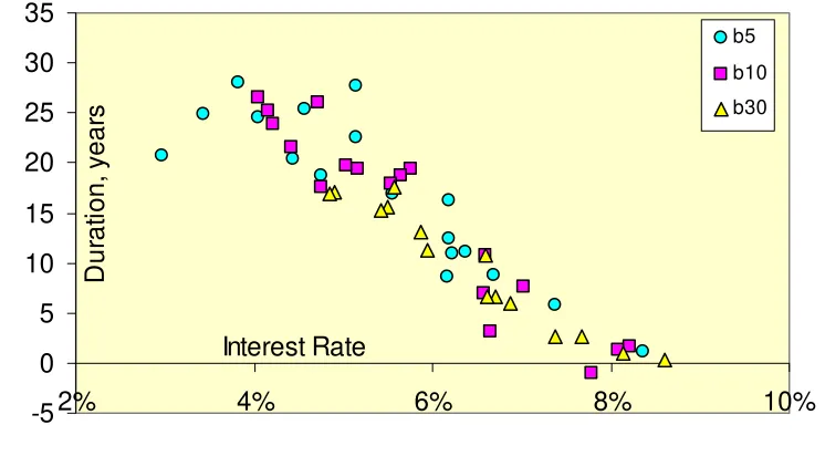
Figure 7 – Plot of the duration of the proposed benchmark, in accordance with the calculation procedure outlined in Table 7. Duration here is shown for different rates, namely b5, b10 and b30,

Figure 7 contains some interesting features. Firstly, the irrelevance principle

discussed earlier seems to apply to duration as well, as the durations computed for the

different rate maturities considered here appear to, more or less, cluster uniformly around

a common trend. This independence of maturity means, for instance, that the duration of

the benchmark relative to b5 would be equal to that relative to b10, if the two rates were to

be the same at a given time, t. This is not surprising because the fundamental input, Φ, into calculating the benchmark’s duration [see Equation 9] is independent of maturity.

Secondly, there seems to be a clear trend that increases with decreasing interest rates,

implying that the overall fall in interest rates, which has been observed since 1990, has

led to a more rate-sensitive benchmark. Since the benchmark’s long-term trend is a

reflection of the major equity indices [i.e. see Figure 5b, for example, for the S&P500], one could conclude that indices have also, on the whole, experienced increased

sensitivity to interest rates since 1990.

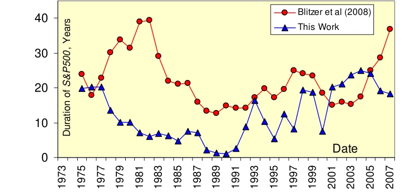
To compare with other works, we display in Figure 8 the duration of the

above-mentioned benchmark plotted alongside that of the S&P500 index, the latter estimated using the method outlined in Blitzer et al _{(2008). The triangles, which summarize the}

outcome of this work, depict the duration values averaged over the three maturities

considered herein, namely b5, b10 and b30.

Figure 8 – Comparison of the duration of the proposed benchmark, as calculated from Equation 9, with that provided in Blitzer et al (2008).

0 10 20 30 40

1973 1975 1977 1979 1981 1983 1985 1987 1989 1991 1993 1995 1997 1999 2001 2003 2005 2007

Blitzer et al (2008)

This Work

D

u

rat

ion

of

S&

P5

0

0

, Ye

a

rs

Prior to comparing the two, we should note that, firstly, the duration estimated in

Blitzer et al _{(2008) relates to S&P500, which has been readily benchmarked here against}

the proposed index, with results shown in Figures 5a-b. Secondly, the method underlying

the reference is based on the DDM, which implements certain assumptions on the risk premium, growth, corporate rating and maturity and, furthermore, incorporates moving

averages and the like.

That said, the two lines in Figure 8 display certain disparities, as well as

similarities. For instance, the estimate of Blitzer et al _{(2008) depicts a rising trend in}

duration during 1977-1981 and 2005-2007, whereas this work shows it to be falling.

With the exception of these relatively short periods, the long-term trends appear to be,

more or less, in line with each other. This goes along with the observation that none of

the curves crosses zero at any point in time14. As for their estimated magnitudes, the

duration measures do seem to correspond better with each other post 1992 rather than

prior to. Altogether, our work shows the GDP-based benchmark to possess a higher volatility, perhaps due to the absence of any averaging scheme, moving and otherwise,

within it.

We now outline another approach to estimating the duration of the newly

proposed benchmark. Returning to Equation 7 and taking its total differential with

respect to time, t, leads to:

t b D b t

S

S

d d d

ln

d _{− =−}

(10)

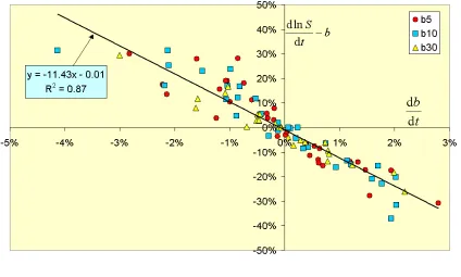
upon combining with Equation 9 and re-arranging. Equation 10 simply states that a plot

of the left-hand side of Equation 10 vs the time rate of change in interest rate, db/dt, all which can be assessed from available data [such as in Table 1], should provide

information on the value of DS. Figure 9 represents exactly this, where b

t S

− d ln d

is

plotted against db/dt over the time period 1975-2008 and for the three maturities

14

considered.15 Without going into any depth, it is noted that a best-fit straight line passing

through all the points has a slope of –11.4, suggesting that the average duration of the

benchmark over the date range and maturities is about 11 years. This value is in good

agreement with the overall average exhibited by the triangles in Figure 8. Equally

important here is the absence of a statistically significant intercept, which is in full accord

with the theoretical form of Equation 10.

Figure 9 – Plot of dlnS/dtvs db/dt over the time period 1975-2008 and for the three maturities considered. According to Equation 10, the slope of the best-fit straight line should represent the

average duration, here being about 11 years.

Finally, we include Figure 10, which is similar to Figure 9 but, for sake of clarity,

focuses on a single maturity and a narrower time frame, namely b10 and 1990-2008,

respectively. The average duration over this time period is estimated at roughly 16 years,

somewhat larger than the overall-average value indicated earlier. The reason for this is

the rising trend in duration after 1990, as observed in Figure 8, and consistent, as well,

thus washing out this statistical anomaly. It should be pointed out that no similar anomalies where observed in relation to any of the other data points throughout the entire time frame 1975-2008.

15

with the data in Figure 7, which portrays an increase in duration with falling interest

rates.

Figure 10 – Same as Figure 9, but focusing only on b10 and the time frame 1990-2008. The

average duration for b10 throughout this time period is shown to be about 16 years. Also, the

absence of a statistically significant intercept is consistent with the form of Equation 10.

Conclusions

This work addresses some of the issues surrounding the direct implementation of the GDP

as a benchmark for broad equity indices and suggests a way for getting around them. It is

shown here that representing the GDP by its underlying value, rather than incorporating it on a standalone basis, produces not only a better fit as a benchmark, but also has other

beneficial uses, such as providing a measure of relative valuation, whereby one could

identify periods of under or over valuation of the index against which the benchmark is

used.

Following on, the benchmark’s duration is investigated as well, offering two

distinctive and objective ways for measuring it, both of which seem to generate

consistent results. While one approach establishes the trend, the other concentrates on

estimating the average over a given time period, leading to the conclusion that the

at about 11 years over the time period 1975-2008, but increases to 16 years over the

period covering 1990-2008. Moreover, the benchmark’s duration appears to have risen

since 1990 as interest rates have fallen gradually, a trend that seems to relate as well to

the duration of the S&P500.

Finally, we re-iterate that this work touches only the surface of this very

important area and, thus, leaves many questions unanswered. For instance, are the

relationships and conclusions derived here universal and applicable equally across

borders and over longer time horizons? Also, could certain situations, where a

connection between the GDP-based benchmark and the underlying equity index is undoubtedly absent, point to underlying data issues or even the possibility of hidden

market manipulations and inefficiencies? An extension of this work could potentially

help address these questions and, perhaps, many others.

References

Blitzer, D.M., S. Dash and P. Murphy (2008) “Equity Duration – Updated Duration of the S&P500”, Standard & Poor’s Publication.

Casabona, P., F. J. Fabozzi, and J. C. Francis (1984) "How to Apply Duration to Equity Analysis", The Journal of Portfolio Management10, pp.52-54.

Cohen, R.D. (2005) “The Relative Valuation of an Equity Price Index,” Chapter 9 in The Best of Wilmott2, P. Wilmott, Ed., John Wiley & Sons, Ltd, pp. 99-132.

Cohen, R.D. (2006) “A Var-based Model for the Yield Curve,” Wilmott Magazine, May issue, pp. 60-68.

Dechow, P.M, R.G. Sloan and M.T. Soliman (2004) “Implied Equity Duration: A New Measure of Equity Risk” Review of Accounting Studies 9, pp. 197-228.

Faugère, C. and J. Van Erlach (2006) “The Equity Premium: Consistent with GDP Growth and Portfolio Insurance”, The Financial Review 41, pp. 547-564.

Honnerová, J. (2003) “Time Series Analysis of GDP and Market Indices”, Bulletin of the Czech Econometric Society 10, pp. 35-64.

Kerschner, E.M., T.M. Doerflinger and D.B. Murphy (1999) “What is the S&P”

PaineWebber Investment Policy report.

Leibowitz, M.L., E.H. Sorensen, R.D. Arnott and H.N. Hanson (1989) “A Total

Differential Approach to Equity Duration”, Financial Analysts Journal 45, pp. 30-37. Santa-Clara, P. (2004) “Discussion of ‘Implied Equity Duration: A New Measure of