http://dx.doi.org/10.4236/jmf.2015.52009
On Two Transform Methods for the
Valuation of Contingent Claims
Chuma Raphael Nwozo1, Sunday Emmanuel Fadugba2 1Department of Mathematics, University of Ibadan, Ibadan, Nigeria
2Department of Mathematical Sciences, Ekiti State University, Ado Ekiti, Nigeria
Email: [email protected], [email protected], [email protected], [email protected]
Received 3 March 2015; accepted 27 March 2015; published 30 March 2015
Copyright © 2015 by authors and Scientific Research Publishing Inc.
This work is licensed under the Creative Commons Attribution International License (CC BY).
http://creativecommons.org/licenses/by/4.0/
Abstract
This paper presents two transform methods for pricing contingent claims namely the fast Fourier transform method and the fast Hilbert transform method. The fast Fourier transform method util-izes the characteristic function of the underlying instrument’s price process. The fast Hilbert transform method is obtained by multiplying a square integrable function f by an indicator func-tion associated with the barrier feature in the real domain. This is also obtained by taking the Hil-bert transform in the Fourier domain. We derived closed-form solutions for European call options in a double exponential jump-diffusion model with stochastic volatility. We developed fast and accurate numerical solutions by means of the Fourier transform method. The comparison of the probability densities of the double exponential jump-diffusion model with stochastic volatility, the Black-Scholes model and the double exponential jump-diffusion model without stochastic volatil-ity showed that the double exponential jump-diffusion model with stochastic volatilvolatil-ity has better performance than the two other models with respect to pricing long term options. An analysis of the fast Fourier transform method revealed that the volatility of volatility σ and the correlation coefficient ρ have significant impact on option values. It was also observed that these parameters
σand ρhave effect on long-term option, stock returns and they are also negatively correlated with volatility. These negative correlations are important for contingent claims valuation. The fast Fou-rier transform method is useful for empirical analysis of the underlying asset price. This method can also be used for pricing contingent claims when the characteristic function of the return is known analytically. We considered the performance of the fast Hilbert transform method and Heston model for pricing finite-maturity discrete barrier style options under stochastic volatility and observed that the fast Hilbert transform method gives more accurate results than the Heston model as shown in Table 3.
Keywords
Merton’s Model, Stochastic Volatility Model, Timer Option
1. Introduction
The Black-Scholes model is the first successful attempt to explain the dynamics of pricing options. But some of its assumptions, like constant volatility or log-normal distribution of underlying price of the asset, do not find justification in the markets. Also strong assumptions in the Black-Scholes model makes it impossible to apply in practice since financial asset returns are not normally distributed. They have fatter tails than the normal distribu-tion proposed and extreme observadistribu-tions are much more frequent in high-frequency financial data. The common big returns that are larger than six-standard deviations should appear less than once in a million years if the Black-Scholes framework were accurate. Squared returns, as a measure of volatility, display positive autocorre-lation over several days, which contradict the constant volatility assumption. Therefore stochastic volatility is needed for option pricing [1]. More complex models, which take into account the empirical facts, often lead to more computations and this time burden can become a severe problem when the computation of many option prices is required. To overcome this problem, Carr and Madan [2] developed a fast Fourier method to compute option prices for a whole range of strikes. This method makes use of the characteristic function of the underlying asset price. The use of the fast Fourier transform method is motivated by the following reasons: The algorithm has speed advantage, this enables the Fourier transform algorithm to calculate prices accurately for a whole range of strikes. The characteristic function of the log-price is known and has a simple form for many models considered in literature while the density is often not known in the closed form. Stochastic volatility can be ob-served in the option markets where smiles and skews in implied volatility occur. These properties lead to more refined models such as Merton, Heston and Bates models [3].
The Black-Scholes model and its extensions constitute the major developments in modern finance. Much of the recent literature on option valuation has successfully applied Fourier analysis to determine option prices such as [4] [5], just to mention a few. These authors numerically solved for the delta and the risk-neutral probability of finishing in-the-money, which can be combined easily with the underlying asset price and the strike price to generate the option value. Unfortunately, this approach is unable to harness the considerable computational power of the fast Fourier transform which represents one of the most fundamental advances in scientific com-puting [6]. Furthermore, though the decomposition of an option price into probability elements is theoretically attractive as explained in Bakshi and Madan [7], it is numerically undesirable due to discontinuity of the pay-offs.
The Bates [8] and Scott [9] option pricing models were designed to capture two features of asset returns namely: the conditional volatility which evolves over time in a stochastic, but mean-reverting fashion and the presence of occasional substantial outliers in asset returns. The Bates and Scott models combined the Heston [10]
model of stochastic volatility with the Merton [11] model of independent normally distributed jumps in the log asset price. The Bates model ignores interest rate risk, while the Scot model allows interest rates to be stochastic. Both models evaluate European option prices numerically, using the Fourier inversion approach of Heston. The Bates model also includes an approximation for pricing American options. The two models are historically im-portant in showing that the tractable class of affine option pricing models includes jump processes as well as diffusion processes.
Zeng et al. [12] considered the pricing of finite-maturity discrete timer options under different types of sto-chastic volatility processes using the fast Hilbert transform algorithms. They also explored the pricing properties of the timer options with respect to various parameters, like volatility of variance, correlation coefficient be-tween the asset price process and instantaneous variance process, sampling frequency and variance budget.
Zeng and Kwok [13] extended the fast Hilbert transform approach for pricing barrier and Bermudian style op-tions under time-changed Levy processes. The success of the fast Hilbert transform approach to compute the fair prices of barrier style derivatives in the Fourier domain lies in the mathematical identity that relates the Fourier transform of a price function multiplied by an indicator function to the Hilbert transform of the Fourier trans-form of the price function. For mathematical backgrounds, transtrans-form methods in the theory of contingent claims and some numerical methods for options valuation see [14]-[35] just to mention a few.
valua-tion of contingent claims.
The paper is outlined as follows: Section 2 gives a brief overview of Bates model in the theory of option pric-ing. Section 3 presents the method of the fast Fourier transform for the valuation of contingent claims. Section 4 presents the fast Hilbert transform method for the valuation of timer options (barrier style options). In Section 5, we present some numerical experiments to illustrate the performance of these transforms. Section 6 concludes the paper.
2. Bates Model
The geometric Brownian motion (Wiener process) is the building block of modern finance. In the Black-Scholes model, the underlying asset price is assumed to follow the dynamics of the geometric Brownian motion of the form:
dSt=rS ttd +σS Wtd t (1) where,
St: the underlying asset price, r: the risk-free interest rate, σ: the volatility, Wt: the Brownian motion or Wiener process and t: the maturity time.
The solution to (1) is obtained as follows; Using the Ito’s lemma
2 2
2
1
d d d
2 t t t t
u u u u
u f g t f W
t S S S
∂ ∂ ∂ ∂
= + + +
∂ ∂ ∂ ∂
(2)
From (1), f =rSt, g=σSt, since the underlying price of the asset St is assumed to follow the process in (1) but we are interested in the process followed by logSt. Let
log t
u= S (3) Differentiating u with respect to the underlying price of the asset St and maturity time t we have
2
2 2
1 1
, , 0
t t t t
u u u
S S S S t
∂ = ∂ = − ∂ =
∂ ∂ ∂ (4)
Substituting (3) and (4) into (2) yields
(
)
2d ln d d
2
t t
S =r−σ t+σ W
(5) Integrating (5) from 0 to t, we have that
2 0exp
2
t t
S =S r−σ t+σW
(6) The empirical facts, however, do not confirm the model assumptions. Financial returns in this model exhibit much fatter tails in other models than in the Black-Scholes model.
Bates proposed a model with stochastic volatility and jumps. This model is the combination of the Merton and Heston models.
2.1. Merton Model
If an important piece of information about a company becomes public it may cause a sudden change in the company’s stock price. To cope with this observation, Merton proposed a model that allows discontinuous tra-jectories of the underlying asset prices. The Merton model is one of the modern pricing models. This model ex-tends (1) by adding jumps to the stock price dynamics, to obtain the modified price dynamics as
identically distributed random variables with mean μ and variance δ2, which are independent of both Nt and Wt. The model becomes incomplete which means that there are many possible ways to choose a risk-neutral meas-ure such that the discounted price process is a martingale. Merton proposed to change the drift of the geometric Brownian motion and to leave the other ingredients unchanged. The underlying price of the asset dynamics is obtained as
2 2
0
1
exp exp 1
2
t
N
t t i
i
S S r σ λ µ δ t σW Y
=
= − − + − + +
∑
(8)Setting
2 2
exp 1
2 M
r δ
µ = −σ −λ µ+ −
(9) The underlying price (8) takes the form
0
1
exp
t
N M
t t i
i
S S µ t σW Y
=
= + +
∑
(10) The jump components add mass to the tail of the returns distribution. Increasing δ adds mass to both tails, while a negative or positive μ implies relatively more mass in the left or right tail. Let the logarithm of the un-derlying price of the asset process be given by0
log t t
S X
S
=
(11) The characteristic function of Xt is of the form;
( )
2 2 2 2Merton
exp exp 1
2 2
Xt
M M
z z
z t σ i z σ i z
ϕ = − + µ +λ − + µ −
(12)
2.2. Heston Model
The Heston model is one of the most widely used stochastic volatility models today. Its attractiveness lies in the powerful duality of its tractability and robustness relative to other stochastic volatility models.
Equation (1) can be modified by replacing the parameter σ with a stochastic process vt which leads to stochastic volatility model with price dynamics given by
dSt =rS ttd + v S Wt td t (13) where vt is the variance process. There are many possible ways of choosing vt.
Hull and White proposed the use of the geometric Brownian motion
1 2
dvt =c v ttd +c v Wtd t (14) However, the geometric Brownian motion tends to increase exponentially as t→ ∞ and this is an undesir-able property for volatility. Volatility exhibits rather a mean reverting behavior. Therefore a model based on an Ornstein-Uhlenbeck-type process:
(
)
dvt=κ θ−vt dt+αdWt (15) was suggested by Stein and Stein [31]. This process, however, admits negative values of the variance vt.
Heston [10] eliminated these deficiencies in the stochastic volatility model by introducing two Brownian mo-tions; 1
t
W in the modified stochastic volatility model in (13) and 2 t
W in the Ornstein-Uhlenbeck-type process (15), and also with the assumption that
Thus (13) reduces to
[ ]
1
d d d
0,
t t t t t
S rS t v S W
t T
= +
∈ (16) and (15) reduce to
(
)
2dvt=κ θ−vt dt+αdWt (17) To obtain the variance process Heston set α σ= vt in (17) to obtain
(
)
[ ]
2
d d d
0,
t t t t
v v t v W
t T
κ θ σ
= − +
∈ (18)
Equation (18) is known as the Heston variance process.
Where St and vt denote underlying price of the asset and volatility processes respectively, Wt1 and 2 t W are correlated with rate ρ. The term vt in (18) simply ensures positive volatility.
As the process reaches the zero bound, the stochastic part becomes zero and the non-stochastic part pushes up the process. The parameter k measures the speed of mean reversion or rate of reversion, θ is the long run mean or the average level of volatility and σ is the volatility of volatility.
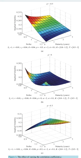
It is clear that, in the Heston model one can implore more than one distribution by changing the value of ρ. We define ρ as the correlation between returns and volatility, and hence we can deduce that ρ affects the heavy tails of the distribution. When ρ<0, there is an inverse proportion between underlying asset price and volatil-ity, when ρ =0, the skewness is close to zero and when ρ>0, this means that as the underlying asset in-creases, volatility increases. The conditions ρ<0, ρ=0 and ρ>0 lead to increase in the heaviness of the right tail and squeezes the left tail as shown inFigure 1(a),Figure 1(b) andFigure 1(c).
The risk neutral dynamics is given in a similar way as in the Black-Scholes model. Taking the exponential of both sides of (11) which have the underlying asset price St as
0e t X t
S =S (19) Using (11) and the fact that σ = vt in (6) we obtain the stochastic differential equation
1
1
d d d
2
t t t t
X =r− v t+ v W
(20) The characteristic function is given by
( )
(
)
(
)
2
2 0
2
0 Heston
2
exp
exp
cosh
cosh sinh 2
2 2
Xt
k t i z
iztr izx
z iz v z
t
i z
t i z t
κθ σ
θ κ ρσ σ
ϕ γ
γ κ ρσ
γ κ ρσ γ
γ
−
+ +
+
= −
− + −
+
(21)
where
(
)
(
)
22 2
z iz i z
γ = σ + + κ− ρσ (22)
x0 is the initial value for the log-price process and v0 is the initial value for the volatility process.
Bates combined the Merton model and Heston model to obtain (Bates model ϕBatesXt
( )
z ≈ϕXHestont( )
z ϕXMertont( )
z ). This model, described in Bates model, adds jumps to the dynamics of the Heston model. For a non-dividend paying stock, the dynamics of the stock price St and its variance vt are given by(
)
1
2
d d d d ,
d d d
t t t t t
t t t t
S rS t v W Z
v κ θ v t σ v W
= + +
{ } { } 0 1, 0.01, 0.04, 0.04, 0.5, 2, 0.1, 0.8 1.2 , 0.5 30
S = r= v = θ= ρ= − κ= σ= K= − T= −
(a)
{ } { }
0 1, 0.01, 0.04, 0.04, 0, 2, 0.1, 0.8 1.2 , 0.5 30
S = r= v = θ= ρ= κ= σ= K= − T= −
(b)
{ } { }
0 1, 0.01, 0.04, 0.04, 0.5, 2, 0.1, 0.8 1.2 , 0.5 30
S = r= v = θ= ρ= κ= σ= K= − T= −
[image:6.595.141.471.74.718.2](c)
(
)
(
)
1
2
d d d d
d d d
t t t t t
t t t t
S r q S t v W Z
v κ θ v t σ v W
= − + +
= − + (24) where q is the dividend yield paid by the underlying asset price St, Zt is a compound Poisson process with inten-sity λ and a log-normal distribution of jump sizes independent of 1
t
W and 2 t
W . If J denotes the jump size then
(
)
(
)
1 2 2log 1 log 1 ,
2
J N χ δ δ
+ = + −
(25) The parameters χ and δ determine the distribution of the jumps and the Poisson process is assumed to be in-dependent of the Brownian motions. Under the risk neutral probability we obtain the equation for the logarithm of the underlying asset price with non-dividend and dividend yields respectively as:
1
1
d d d
2
t t t t t
X =r−λχ− v t+ v W +Z
(26)
1
1
d d d
2
t t t t t
X =r− −q λχ− v t+ v W +Z
(27)
where Zt is a compound Poisson process with normal distribution of jump magnitudes.
Since jumps are independent of the diffusion part in Equation (23), then the characteristic function for the log-price process in which the underlying asset price pays no dividend is obtained as:
( )
(
)
(
)
(
)
(
)
2 2 0 2 0 Bates 22 2 2
exp
exp
cosh
cosh sinh 2
2 2
exp exp log 1 1
2 2
Xt
k t i z
izt r izx
z iz v z
t
i z
t i z t
z t
κθ σ
θ κ ρσ λχ
σ
ϕ γ
γ κ ρσ
γ κ ρσ γ
γ δ δ λ χ − + − + + = − − + − + × − + + − − (28)
Similarly, for dividend paying stock we have:
( )
(
)
(
)
(
)
(
)
2 2 0 2 0 Bates 22 2 2
exp
exp
cosh
cosh sinh 2
2 2
exp exp log 1 1
2 2
Xt
k t i z
izt r q izx
z iz v z
t
i z
t i z t
z t
κθ σ
θ κ ρσ
λχ σ
ϕ γ
γ κ ρσ
γ κ ρσ γ
γ δ δ λ χ − + − − + + = − + − + − × − + + − − (29)
Equations (28) and (29) can be written in the form
( )
t
Bates
X z D J
ϕ = + , since they can be split into diffusion part D and jump part J. Therefore, we have respectively for (28) and (29) below
( )
(
)
(
)
(
)
(
)
2 2 0 2 0 Bates 22 2 2
exp
exp
cosh
cosh sinh 2
2 2
exp exp log 1 1
2 2
t
X
k t i z
izt r izx
z iz v z
t
i z
t i z t
z t
κθ σ
θ κ ρσ λχ
σ
ϕ γ
γ κ ρσ
γ κ ρσ γ
and
( )
(
)
(
)
(
)
(
)
2
2 0
2
0 Bates
2
2 2 2
exp
exp
cosh
cosh sinh 2
2 2
exp exp log 1 1
2 2
t
X
k t i z
izt r q izx
z iz v z
t
i z
t i z t
z t
κθ σ
θ κ ρσ
λχ σ
ϕ γ
γ κ ρσ
γ κ ρσ γ
γ
δ δ
λ χ
−
+ − − +
+
= −
+ − + −
+ − + + − −
(31)
In Equation (30), we observe that the diffusion part is similar to (22) with difference of λχ called risk neu- tral correction. Also (12) has a similar structure as the jump part in (30), where
(
)
2
log 1
2 δ
µ= +χ − . Since the jumps are assumed to be independent, the characteristic function is the product of Heston model Heston
( )
t
X z
ϕ and
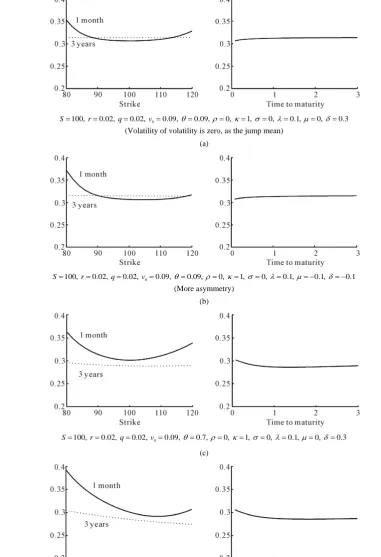
the jump part in (30).Figure 2 shows that adding jumps makes it easier to introduce curvature into the volatility surface, at least for short maturities.
Remark 1:
Assuming that the previous dynamics represent the evolution of the state process
(
S vt, t)
under a risk-neu- tral measure, then the pricing equation of a European contingent claim c on S is given by(
)
(
)
2 2 2
2 2
2 2
1 1
0
2 2
c c c c C c
vS v vS r q S v rc c
t S σ v ρθ S v λχ S κ θ v ψ
∂ + ∂ + ∂ + ∂ + − − ∂ + − ∂ − + =
∂ ∂ ∂ ∂ ∂ ∂ ∂ (32)
where
(
)
(
) (
) ( )
( )
(
)
(
)
0
2 2
2
2
, , , , , , d
1 1
exp log
2 2π
1 : log 1
2 : exp
2
c S v t c S v t c S v t g
g m
m k
m
ψ λ ξ ξ ξ
ξ ξ
δ δξ
χ δ
δ
∞
= −
= − −
= + −
=
+
∫
(33)
Equation (32) holds for S∈
[
0,∞)
, with the assumption that v∈[
0,vmax]
. The partial differential equation is usually given along with a proper payoff. In the case of vanilla European call option we have that:( ) (
,)
max(
, 0)
c S v = S−K + = S−K (34) where K is the strike price or exercise price. It should be noted that closed form solutions of problem (32) for vanilla-option payoff do exist. Nevertheless, direct numerical integration of (32) is important when dealing with non-trivial payoff functions.
3. Fast Fourier Transform Method in the Theory of Contingent Claims
This section presents some fundamental properties of Fourier transform and the fast Fourier transform method for the valuation of European options.
3.1. Fourier Transform
The Fourier transform is a generalization of the complex Fourier series and is given by
( )
(
)
( )
( )
( )
e2πikxdF f x k f k f x x
∞ −
∞
0
100, 0.02, 0.02, 0.09, 0.09, 0, 1, 0, 0.1, 0, 0.3
S= r= q= v = θ= ρ= κ= σ= λ= µ= δ=
(Volatility of volatility is zero, as the jump mean)
(a)
0
100, 0.02, 0.02, 0.09, 0.09, 0, 1, 0, 0.1, 0.1, 0.1
S= r= q= v = θ= ρ= κ= σ= λ= µ= − δ= −
(More asymmetry)
(b)
0
100, 0.02, 0.02, 0.09, 0.7, 0, 1, 0, 0.1, 0, 0.3
S= r= q= v = θ= ρ= κ= σ= λ= µ= δ=
(c)
0
100, 0.02, 0.02, 0.09, 0.7, 0.3, 1, 0, 0.1, 0.1, 0.3
S= r= q= v = θ= ρ= − κ= σ= λ= µ= − δ=
[image:9.595.108.490.89.647.2](d)
where
( )
( )
2π( )
( )
2πe ikxd and e ikxd
f x f k k f k f x x
∞ ∞
−
−∞ −∞
=
∫
=∫
(36)are square integrable and characteristic functions respectively. In the form (35) we have the forward (−i) Fourier transform. The inverse (+i) Fourier transform is given by
( )
(
)
( )
( )
( )
1 1 2π
e d
2π
ikx
F f k x f x f k k
∞ −
−∞
= =
∫
(37)
Some Fundamental Properties of Fourier Transforms
Let the Fourier transform of f x
( )
be defined as F f x(
( )
)
= f k( )
then the following fundamental properties hold as follows:• Scaling Property
( )
(
)
( )
e2πikd 1 kF f cx f cx x f
c c ∞ − −∞ = =
∫
(38)• Shifting/Translation Property
(
)
(
)
(
)
( )
( )( )
( )
0 0 0 2π 2π 02π 2π 2π
e d e d
e e d e
ik u x ikx
ikx iku ikx
F f x a f x x x f u x
f u u f k
∞ ∞ − + − −∞ −∞ ∞ − − − −∞ − = − = = =
∫
∫
∫
(39)• Fourier Transform of Derivatives
( ) ( )
(
) ( )
2π( )
d
2π e d 2π
d
ikx
F f x k ik f x x ikf k
x ∞ − −∞ = =
∫
(40)This process can be iterated for the nth derivative to yield
( ) ( )
(
) ( )
2π(
) ( )
d 2π
e d 2π
d n
n ikx n
n
F f x k ik f x x ik f k
x ∞ − −∞ = =
∫
(41)Thus, a differentiation converts to multiplication in Fourier space. • Convolution Property
( ) ( )
(
)
( )
( ) (
)
( )
(
)
(
( )(
)
)
( )
(
)
(
( )(
)
)
( )
(
)
(
( )
)
( ) ( )
2π 2π 2π 2π 2πe d d
e d e d
e d e d
ikx
ik x x ikx
ik x x ikx
F f x g x k f x g x x x x
f x x g x x x
f x x g x x x
F f x F g x f k g k
∞ ∞ − −∞ −∞ ∞ ∞ ′ − − ′ − −∞ −∞ ∞ ∞ ′ − − ′ − −∞ −∞ ′ ′ ′ ∗ = − ′ ′ ′ = − ′ ′ ′ = − = =
∫ ∫
∫ ∫
∫
∫
(42) Similarly,( ) ( )
(
)
( ) ( )
F f x g x = f k ∗g k (43) • Linear Property
( )
( )
(
)
( )
(
( )
( )
)
( )
( )
( )
( )
2π 2π 2π e de d e d
ix
ix ix
F af x bg x k af x bg x x
a f x x b g x x af k bf k
3.2. The Fast Fourier Transform
The fast Fourier transform is an efficient algorithm for computing the discrete Fourier transform of the form;
( )
11
2π
exp , 1, 2, 3, , N
j j
i
m p pj x p N
N
−
=
−
= =
∑
(45)where N is typically a power of two. Equation (45) reduces the number of multiplications in the required N
summations from an order of N2 to that of Nln2
( )
N , a very considerable reduction. Let p and j be written as binary numbers i.e. p=2p1+ p0 and j=2j1+ j0 with j j1, 0,p p1, 0∈{ }
0,1 , then (45) becomes(
)
(
)(
)
( )( )( )
( ) ( ) ( )
1 0 0 1
1 0 1 0 0 1 0 1 0
1 0 1 0
0 1 0 1
1 1
1 0 1 0 1 0 ,
0 0
1 1 1 1
2 2 2 2
, ,
0 0 0 0
2π
, exp 2 2 j j
j j
p p j j p j j p p
j j j j
j j j j
i
m p p p p j j x
N
A x A A x
= =
+ + +
= = = =
−
= + +
= =
∑ ∑
∑ ∑
∑ ∑
(46)The fast Fourier transform can be described by the following three steps as
(
)
( )(
)
(
)
( )(
)
(
)
0 1 0 1 1
0 1 0
1
1
2 1
0 0 ,
0 1
2
2 1
0 0 0 0
0 2
0 1 0 1
,
, ,
, ,
p j j j j
j p p
j
m p j x A
m p j m p j A
m p p m p p
=
+
=
=
=
=
∑
∑
(47)The basic idea of the fast Fourier transform is to develop an analytic expression for the Fourier transform of the option price and to get the price by means of Fourier inversion.
The Fast Fourier Transform Method for the Valuation of European Call Option
The Fast Fourier transform method is a numerical approach for pricing options which utilizes the characteristic function of the underlying instrument’s price process. The Fast Fourier transform method assumes that the characteristic function of the log-price is given analytically.
Consider the valuation of European call option. Let the risk neutral density of S=logST be fT
( )
ST . The characteristic function of this density is given by( )
e2πivS( )
dT v f S S
ϕ ∞ −
−∞
=
∫
(48)The price of a European call option with maturity T and exercise price K denoted by CT
( )
p is given by( )
exp(
)
(
eS)
( )
d Tp
C p rT K f S S
∞
=
∫
− − (49)where p is the log of the strike price Ki.e.
e
log ep
p= K⇒K= (50) Substituting (50) into (49) yields
( )
exp(
)
(
eS ep)
( )
d Tp
C p rT f S S
∞
=
∫
− − (51)( )
(
)
(
)
( )
0lim T lim exp eS ep d
k k
p
C p rT f S S S
∞
→−∞ →−∞
= − − =
∫
(52)( )
e p( )
, 0T T
c p = α C p α > (53) Equation (53) is square integrable in p over the entire real line. Using (36) and (37), we have that
( )
(
)
( )
e2πikp( )
dT T
F c p c k c p p
∞ −
−∞
= =
∫
(54)( )
(
)
( )
( )
1 1 2π
e d
2π ikp
T T
F c p c p c k k
∞ −
−∞
= =
∫
(54a)Substituting (54a) into (53) and solving further, then we obtain a new call value given by
( )
2π( )
2π( )
0
1 1
e e d e e d
2π π
p ikp p ikp
T T T
C p α c k k α c k k
∞ ∞
− − − −
−∞
=
∫
=∫
(55)
(56) is a direct Fourier transform and lends itself to an application of fast Fourier transform method. (54) is computed as follows:
( )
(
)
(
)
( )
( )
(
(
)
)
( )
(
(
)
)
( )
(
( ))
(
( ))
2π 2π 2π 2π 2πe exp e e d d
e e e e e d d
e e e e e d d
e e
e e e d
2π 2π 1
ikp S p
T
p
rT p S p ikp
p
rT p S p ikp
p
S S S S
ik p ik p
rT
c k rT f S S p
f S S p
f S p S
f S S
ik ik α α α α α α ∞ ∞ − −∞ ∞ ∞ − − −∞ ∞ ∞ − − −∞ ∞ + + − −∞ −∞ −∞ = − − = − = − = − + + +
∫
∫
∫
∫
∫
∫
∫
(56)Since lim e( 2πik p) 0 p
α +
→−∞ = with α >0, then the last equation in (56) becomes
( )
( )
(
)
(
)
( )
(
(
)(
)
)
(
)
(
)
(
)
2 2 2
exp 1 2π exp 1 2π
e d
2π 1 2π
exp 1 2π
e d
2π 1 2π
e 2π 1
4π 2π 2 1
rT T
rT
rT T
ik S ik S
c k f S S
ik ik
ik S
f S S
ik ik k i k ki α α α α α α α ϕ α
α α α
∞ − −∞ ∞ − −∞ − + + + + = − + + + + + = + + + − + = + − + +
∫
∫
Finally we have
( )
(
(
)
)
(
)
2 2 2
e 2π 1
4π 2π 2 1
rT T T
k i
c k
k k i
ϕ α
α α α
− − +
=
+ − + +
(57)
Setting v=2πk, then (57) becomes
( )
2(
2(
(
)
)
)
e 1 2 1 rT T T v i c v
v v i
ϕ α
α α α
− − +
=
+ − + +
(58)
The corresponding put values can be obtained by defining
( )
e p( )
T T
p p = −α P p , v=2πk, α >0 with Fou-rier transform
( )
2(
2(
(
)
)
)
e 1 2 1 rT T T v i p v
v v i
ϕ α
α α α
− − − +
=
− − + − +
(58a)
given by cT
( )
0 being finite. This is equivalent to EQ( )
ST 1α + < ∞
. Substituting (58) into (56) with v=2πk, we have
( )
2(
2(
(
)
)
)
0
e 1
1
e e d
π 2 1
rT T
p ivp
T
v i
C v v
v v i
α ϕ α
α α α
− ∞ − − − + = + − + +
∫
(59)Similarly, for the price of put option we have that:
( )
2(
2(
(
)
)
)
0
e 1
1
e e d
π 2 1
rT T
p ivp
T
v i
C v v
v v i
α ϕ α
α α α
− ∞ − − − − + = − − + − +
∫
(59a)For the put formula to be well defined, is suffices to choose an appropriate α >0 in a way that
( )
Q T
E S−α <∞.
The European call values are calculated using (59). Carr and Madan [2] established that if α =0 the de-nominator of (59) vanishes when v = 0, inducing a singularity in the integrand. Since the fast Fourier transform evaluates the integrand at v = 0, the use of the factor eαp is required.
Now, we obtain the desired option price in terms of cT using Fourier inversion of the form:
( )
( )
0
1
e e d
π
p ivp
T T
C p α c v v
∞
− −
=
∫
(60)
Using basic trapezoidal rule, (60) can be computed numerically as:
( )
1( )
0 1 e e π N p ivp
T T j
j
C p α c v η
−
− −
=
=
∑
(61)
where
, 0,1, 2, 3, , 1, 0
j j
v =η j= N− η> (62) We are interested in (at the money call values) CT
( )
p
, the case where the strikes near the underlying spot price of the asset. This type of options is traded most frequently. The fast Fourier transforms method returns N
values of p and we then consider a uniform spacing of size >0 for the log-strikes around the log-spot price
S0 of the form:
, 0,1, 2, , 1 u
k = +a u u= N− (63) Equation (63) gives us log-strike levels ranging from −a to a, where
2
N
a= − (64) Substituting (63) and (64) into (61), we have
( )
1( )
0
1
exp exp
2 π 2
N
T u T j
j
N N
C k α u iv u c v η
− = − = − − +
∑
(65)
Now, the fast Fourier transforms method can be applied to xi in (45) provided that 2π
N
η =
. Hence the inte- gration (60) is an application of the summation (45).
Remark 2:
• For an accurate integration with larger values of η we apply basic Simpson’s 1
3 rule weightings into (65)
with the condition 2π
N
η =
, then the accurate call price which is the exact application of the fast Fourier transform method is obtained as:
( )
1( )
(
( )
)
1 0
1 2π
exp exp 3 1
2 π 3
N
j
T u j T j j
j
N i
C k u u iav c v
N
η
α − δ −
= − = − + + − −
∑
where ku= +a ρu, u=0,1, 2,,N−1 and δj is called the Kronecker delta function expressed as: 0, if 0
1, if 0 j
j j
δ = ≠=
(67) • For in-the-money and at-the-money options prices, call values are calculated by an exponential function to obtain square integrable function whose Fourier transform is an analytic function of the characteristic func-tion of the log-price. Unfortunately, for very short maturities, the call value approaches to its non-analytic intrinsic value causing the integrand in the inversion formula of Fourier transforms to vary above and below a mean value and therefore remains tedious to be integrated numerically. We use the alternative approach called the “Time Value Method” proposed by Carr and Madan [2] to mitigate this numerical inconvenience. This approach works with time values only, which is quite similar to the previous approach. But in this con-text the call price is obtained by means of the Fourier transform of a modified time value, where the modifi-cation involves a hyperbolic sine function instead of exponential function.
Let zT
( )
k represent the time value of out-of-the-money (OTM), that is, for S<k we have the call price for zT( )
k and for S>k we have the put option for zT( )
k . Setting S0 =1 for simplicity, zT( )
k is de-fined by( )
e(
e e)
, 0( )
d e(
e e)
, 0( )
drT S k rT S k
T k S k k S k
z k f S S f S S
∞ ∞
− −
> < < >
−∞ −∞
=
∫
− Ι +∫
− Ι (68)where f S
( )
is the risk-neutral density of the log-price S and I denotes the indicator function. Let the Fourier transform of zT( )
k be defined by( )
eivk( )
dT v zT k k
υ ∞
−∞
=
∫
(69)The prices of OTM options can be obtained by the inversion formula of the Fourier transform of (69) of the form
( )
eivk( )
dT T
z k υ v v
∞ −
−∞
=
∫
(70)By substituting (68) into (69) and writing in terms of characteristic functions then (69) becomes
( )
(
)
( )
(
)
( )
( )
(
)
(
)
, 0 , 0
e e e e d e e e d d
e e
e
1 1
ivk rT S k rT S k
T k S k k S k
rT rT
rT
T T
v S S f S S k
i v i
iv iv iv iv
υ
ϕ ϕ
∞ ∞ ∞
− −
> < < >
−∞ −∞ −∞
− −
−
= − Ι + − Ι
− −
= − −
+ +
∫
∫
∫
(71)
There are no issues regarding the integral of this function in (71) as k→ −∞ or ∞, the time value at k tends to zero can get rather steep as T tends to zero and this can make the Fourier transform to be wide and oscillatory. By considering the damping function sinh
( )
αk , the time value follows a Fourier inversion:( )
1( )
( )
e d
πsinh
ivk
T T
z k v v
k ζ
α
∞ −
−∞
=
∫
(71a)where
( )
e sinhivk( ) ( )
dT v k zT k k
ζ ∞ α
−∞
=
∫
(72)Solving (72) further and replace sinh
( )
αk by e e 2k k
α − −α
, then we have
( )
e e( )
(
)
(
)
e d
2 2 2
k k
T T
ivk
T T
v i v i
v z k k
α α υ α υ α
ζ ∞ −
−∞
+ −
−
= = − −
The use of the fast Fourier transform for calculating out-of-the-money option prices is similar to (66). The only differences are that they replace the multiplication by
(
)
(
(
)
)
exp exp exp
2 u
N
k a u ρ u
α α ρ α ρ
− = − + = −
with a division by sinh
( )
αk and the function call to cT( )
vj be replaced by a function ζT( )
v . Hence the formula for out-of-the-money option price is given by( )
(
)
(
)
1( )
(
( )
)
1 0
1 2π
exp exp 3 1
πsinh 3
N
j
T u u j T j j
j u
i
C k k u iav v
k N
η
α ζ δ
α − − = − = − + + − −
∑
(74) where 2 u Nk = +a ρu= ρ−ρu
, u=0,1, 2,,N−1 and δj is called the Kronecker delta as given by (67).
3.3. A Closed Form of European Option Pricing under Double Exponential Jump-Diffusion Model with Stochastic Volatility
We derive a closed-form solution of a European call option pricing under double exponential jump-diffusion model with stochastic volatility. The corresponding European put option can be obtained easily by means of put- call parity. For this purpose, we need the following results.
Lemma 3.3.1
Suppose that the variance process vt follows a square root process of the form:
(
)
0 0dvt = θ κ− vt dt+σ v Wtd t, vt =v (75) and s1, s2 are any complex, one has
( )
( )
( )
(
( ))(
)
( )
(
)
(
(
)
)(
(
)
)
1 0 0 0.5 2 2 21 2 2
2 2
2 2
1
exp d exp
2 2 e
log
2 e 1 e
1 e 2 1 e
2 e 1 e
2 T
t t t
T
T T
T T
T T
E s v t s v A T B T v
A T
s
s s s
B T s s κ γ γ γ γ γ γ γ θ γ
σ γ κ γ σ
κ γ
γ κ γ σ
γ κ σ
− − − − − − − − − = − = + + + − − − + − = + + + − = +
∫
(76) Remark 3:This result shows that (76) holds because of the affine structure of the variance process.
Lemma 3.3.2 [13]
Suppose the underlying price of the asset follows:
1 1
1 2
log 1
1 1
t t t t
p q
S X λt η η rt ξ ς
η η
= − + − + + +
− +
(77)
and z is any complex, then
(
)
(
)
(
)
( )
(
)(
)
(
)
(
(
)
)(
(
)
)
1 1 1 1
1 2 1 2 0
0.5
1 2 2
2 2 2
2 2
exp log
exp 1 1 1
1 1
1 e 2 1 e
2 2 e
log
2 e 1 e 2 e 1 e
T
T
T T
T
T T T T
E rt z S
p q p q
z rT T z T z V T
z z
s s s
s s
γ γ
κ γ
γ γ γ γ
η η η η ρσ
λ λ θ
η η η η σ
κ γ
θ γ
σ γ κ γ σ γ κ γ σ
− − − − − − − − + = − + + − − + − − + − + − + − − + − + + + + + − + + + −
0
(
)
(
2)
2 2 20 0 0 0
1 2
1 1
,
2 2
z z z
s ρ σ z ρσ κ ρ σ s ρσ
σ σ
− − −
= − − = −
Lemma 3.3.3 [35]
Suppose ϕu= Eexp
(
iulogSt)
is the characteristic function of logSt, then(
)
(
)
(
)
2 2 0 2 01 1 1 1
0
1 2 1 2
2
exp log
2 1 e
1 1
1 1
u T t
T iu T
iu S iu
p q p q
T iu iurT v
iu iu
θ σ
δ
θ κ δ θσ ρ
δ ϕ
σ σ
δ κ δ ρσσ
η η η η
λ ε
η η η η
− − = × + − + − − − + − + + − − − + + − + + (79) where
(
)
(
)
(
)
(
)
(
)
(
)
2 2 2
0 0
2
0
1 1 1 e
2 1 e
T
T
iu iu iu
iu iu iu
δ
δ
δ κ ρσσ σ σ
σ ε
δ κ δ ρσσ
− − = − + − − − = + − − − (80) Theorem 3.3.4
Let k denote the log of the strike price K, xT =logST and CT
( )
k the desired value of a T-maturity call op-tion with strike ek. Assume that, under martingale probability measure P*, the underlying asset price St with dividend paying stock q and its components are given by:(
)
(
)
( )
0 1 1 01 1 0 2 2 0 1 2
1 1 2 1
1 2 1 2
1 1 2 1
d d d
d d d ,
e e , , 0
exp 1 , , 0, 1
c c c
t t t t t
t t t t t
y y
y y
t t
c t t t
S r q S t v S W
v v t v W v v
f y p p
p p
J x t p p p p
S S J
η η
γ
σ
θ κ σ
η η η η
η η λ η η − − ≥ < − + = − + = − + =
= Ι + Ι >
= − + − > + =
=
(81)
( )
uϕ is the characteristic function of xT, h x
( )
is the probability density of xT given by( )
2π( 1)( 1)( )
1
1
e , 1, ,
π
N i j k
N
j
h x ϕ u k N
− − −
=
=
∑
= (82)then the initial call value CT
( )
k is written as( )
(
)
(
)
( )
0
e 1 e
1 1
e e e e d
2 π
iuk iuk
T T
qT rT qT rT
T t t
u u
C k S K S K u
iu iu
ϕ ϕ
∞
− − − − −
= − + ℜ − ℜ
∫
(83)where ℜ ⋅
[ ]
represents the real part.Proof:
From the risk-neutral theory, we have for the case of dividend yield q, the call price of the form
( )
(
)
(
)
( )
(
)
( )
0
1 2
e e e e d
e e eT d e e
rT rqT rT qT
T t t t t
x
rT qT qT rT
k
C k E S K S K h S S
K h x x S
∞ + + − − − − ∞ + − − − − = − = −
= − = Π − Π
∫
∫
(84)
get
d e
d e
T T
x
x
Q
P E
∗
∗ =
We can write that
(
)
( )
eiuxTQ u i
E
u
ϕ ϕ
∗ −
=
(85) Because of the no-arbitrage condition, we can obtain
(
)
( )
1
0
e 1 1
d 2 π
iuk T
T
u i u iu i
ϕ ϕ
−
∞ −
Π = + ℜ −
∫
(86)From the Fourier transform formula, the probability density for this model is given by
( )
( )
0
1
e d
π iuk
h x ϕ u u
∞ −
=
∫
(87)Hence,
( )
2
0
1
e d d
π iuk
k
u u x
ϕ
∞ ∞
−
Π =
∫ ∫
(88)Therefore, (88) becomes
( )
2
0
e 1 1
d 2 π
iuk T u
u iu
ϕ
−
∞
Π = + ℜ
∫
(89)From (84), (86), (89) and (96), we can obtain the required Theorem 3.3.4.
Remark 4:
For the of non-dividend yield, see [35].
4. Fast Hilbert Transform in the Theory of Contingent
The Hilbert transform of integrable function f is well defined by the following Cauchy principal value integral
( )
(
)
1(
( )
)
d π
f y
H f x PV y
x y
∞
−∞
=
−
∫
(90)Let the Fourier transform of f be defined as
( )
(
( )
)
( )
ei xdf ψ F f x f x ψ x
∞ ∗
−∞
= =
∫
(91)Suppose that f∗ is also integrable, a well-known identity in Fourier analysis that is crucial for the applica-tion of Hilbert transform is the following;
(
sgn)( )
( )
F f ⋅ ψ =iHf∗ ψ (92) Here sgn
( )
x is a signum function defined by( )
1, 0Sgn 0, 0
1, 0
x
x x
x
− <
= =
>
(93)