Evaluating the performance of convolutional neural networks with direct acyclic graph architectures in automatic segmentation of breast lesion in US images

(1)

R E S E A R C H A R T I C L E

Open Access

Evaluating the performance of

convolutional neural networks with direct

acyclic graph architectures in automatic

segmentation of breast lesion in US images

Marly Guimarães Fernandes Costa

1

, João Paulo Mendes Campos

1

, Gustavo de Aquino e Aquino

1

,

Wagner Coelho de Albuquerque Pereira

2

and Cícero Ferreira Fernandes Costa Filho

1*

Abstract

Background:Outlining lesion contours in Ultra Sound (US) breast images is an important step in breast cancer diagnosis. Malignant lesions infiltrate the surrounding tissue, generating irregular contours, with spiculation and angulated margins, whereas benign lesions produce contours with a smooth outline and elliptical shape. In breast imaging, the majority of the existing publications in the literature focus on using Convolutional Neural Networks (CNNs) for segmentation and classification of lesions in mammographic images. In this study our main objective is to assess the ability of CNNs in detecting contour irregularities in breast lesions in US images.

Methods:In this study we compare the performance of two CNNs with Direct Acyclic Graph (DAG) architecture

and one CNN with a series architecture for breast lesion segmentation in US images. DAG and series architectures are both feedforward networks. The difference is that a DAG architecture could have more than one path between the first layer and end layer, whereas a series architecture has only one path from the beginning layer to the end layer. The CNN architectures were evaluated with two datasets.

Results:With the more complex DAG architecture, the following mean values were obtained for the metrics used

to evaluate the segmented contours: global accuracy: 0.956; IOU: 0.876; F measure: 68.77%; Dice coefficient: 0.892. Conclusion:The CNN DAG architecture shows the best metric values used for quantitatively evaluating the segmented contours compared with the gold-standard contours. The segmented contours obtained with this architecture also have more details and irregularities, like the gold-standard contours.

Keywords:Breast lesion, Ultrasound images, Convolutional neural networks

Background

Breast cancer is one of the leading causes of death among women under 40 years old [1]. According to the World Cancer Report, 2018, lung and female breast cancers are the leading types worldwide in terms of the number of new cases of cancers among women [2]. Studies have shown that detection of early-stage breast cancers, followed by appropriate treatment, was

responsible for a 38% drop in the mortality rate from 1989 to 2014 [1]. Digital mammography (DM) and Ultrasound (US) are two commonly used techniques for breast lesion detection [3]. Although DM is considered the most effective technique [3], US imaging has the advantage of being safer, more versatile and sensitive to lesions located in dense areas, normally found in young women, and where lesions have an attenuation similar to the dense tissue. Therefore, they can be hidden by the surrounding tissue [4]. US imaging is heavily dependent on radiologist experience, compared to DM.

Outlining lesion contours in US breast images is an important step in breast cancer diagnosis. Malignant

© The Author(s). 2019Open AccessThis article is distributed under the terms of the Creative Commons Attribution 4.0 International License (http://creativecommons.org/licenses/by/4.0/), which permits unrestricted use, distribution, and reproduction in any medium, provided you give appropriate credit to the original author(s) and the source, provide a link to the Creative Commons license, and indicate if changes were made. The Creative Commons Public Domain Dedication waiver (http://creativecommons.org/publicdomain/zero/1.0/) applies to the data made available in this article, unless otherwise stated.

* Correspondence:[email protected] 1

Centro de Tecnologia Eletrônica e da Informação/Universidade Federal do Amazonas, Av. General Rodrigo Otávio Jordão Ramos, 3000, Aleixo, Campus Universitário_–Setor Norte, Pavilhão Ceteli, Manaus, AM CEP: 69077-000, Brazil

(2)

lesions infiltrate the surrounding tissue, generating irregu-lar contours, with spiculation and angulated margins, while benign lesions produce contours with a smooth out-line and elliptical shape [4]. On the other hand, low-contrast images associated with speckle noise generate spurious borders hampering lesion outline and hinder accurate diagnosis.

Spurred on by the success of machine learning and image processing in computer vision applications, many attempts have been made to build Computer-Aided Diag-nosis (CAD) systems for breast lesion segmentation [5–9]. Daoud et al. [5] used support vector machines with texture input variables, for segmenting breast lesions in US images. The dataset consists of 50 breast US images with sizes of 418 × 566 pixels. The authors obtained the following results: True Positive Fraction = 91.13% ± 4.06%, False Positive Fraction = 8.87% ± 4.06% and False Negative Fraction = 15.58% ± 7.13%. In [6], a different approach was taken, using graph cuts and level set. However, the authors do not present quantitative results. In Jiang et al. [7], the authors used the algorithm of ran-dom walks to breast lesion segmentation in a dataset with 112 US images segmented by medical specialists. The authors obtained the following results: Accuracy = 87.5%, Sensitivity = 88.8% and Specificity = 84.4%. In [8], the dataset consists of only of 30 images and the authors used self-organized maps associated with finite impulse response filters for breast US images segmentation. The authors obtained the following results: True Positives (TP) = 93.24%, False Positives (FP) = 8.41% and Intersec-tion over Union (IoU) = 86.95%. In [9], the authors used fuzzy histogram equalization for improving the US image contrast and the random forest classifier for breast lesion segmentation. The authors do not present quantitative results.

Considering the huge popularity of Deep Learning and, in particular, of CNNs in segmenting and classify-ing objects, the followclassify-ing question naturally arises: Can a CNN, using a relatively small dataset, such as those available in medical datasets, outperform traditional machine learning techniques in segmentation of breast tumors in US imaging?

According to Yap et al. [10], in breast imaging, a large number of recent publications concentrate on using CNNs for mammography. Dhungel et al. [11] addresses the problem of mass segmentation using deep learning; Mordang et al. [12] used CNNs in microcalcification de-tection. Recently, Ahn et al. [13] address the problem of breast density estimation using CNNs. Only the study of Yap et al. [10] focuses on CNNs for automatic segmen-tation of breast lesions in US images. The authors compared the performance of three CNN architectures, Le-Net [14], U-Net [15] and Fully Convolutional Net-work (FCN) Alex-Net [16] with three machine learning

techniques, Rule-Based Region Ranking, Multifractal Fil-tering and Radial Gradient Index filFil-tering. Two datasets, dataset A with 306 breast US images and dataset B with 163 breast US images were used in this comparison. Ac-cording to the authors, considering the parameters false positives/image and F-measure, FCN-AlexNet obtained the best performance for dataset A and the Patch-based LeNet achieved the best performance for Dataset B. The authors conclude that the CNN architectures evaluated outperform traditional machine learning techniques in breast lesion segmentation in US imaging.

In this study our main objective is to assess the ability of CNNs in detecting contour irregularities in breast le-sions in US images. With this aim, we propose two CNNs with DAG architectures and compare the per-formance of these proposed architectures with a pro-posed series architecture. DAG and series architectures are both feedforward networks. The difference is that a DAG architecture could have more than one path from the first layer and end layer, while a series architecture has only one path from first layer to end layer. When ap-plied to image processing, DAG architectures aggregate information of pixel localization contained in initial layers into final layers. In semantic tasks, it is expected that this procedure enhances fine image details. There-fore, it is expected that DAG architectures will improve breast lesion segmentation in US images.

Methods

Work environment

Experiments were performed in Matlab 2017b

(9.3.0.713579). The computer used was equipped with a DELL® motherboard with 128 GB RAM, a Intel® Core™ i5-7200U CPU @ 2.50GHz. The graphics pro-cessing unit used was a Nvidia GeForce 940MX, with 4GB RAM and 384 CUDA cores. The computer oper-ating system was Windows 10.

Input dataset

(3)

Dataset B was collected in 2012 from the UDIAT Diag-nostic Centre of the Parc Taulí Corporation, Sabadell (Spain) with a Siemens ACUSON Sequoia C512 system 17 L5 HD linear array transducer (8.5 MHz). The dataset con-sists of 163 images from different women with different image sizes. Within the 163 lesion images, 53 were images with cancerous masses and 110 with benign lesions [10].

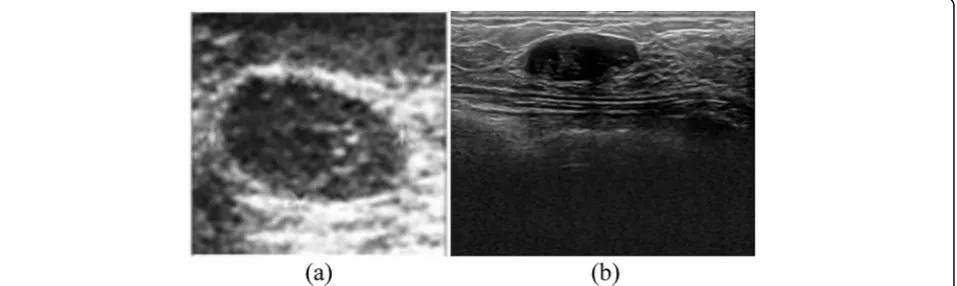
Due to hardware limitations, all images of both data-bases were resized to 160 × 160 pixels or to 320 × 320 pixels. We evaluated the following sets: Dataset A: cropped image resized to 160 × 160; Dataset B: cropped image resized to 160 × 160, original image resized to 160 × 160, original image resized to 320 × 320.

Figure 1a shows an original image from dataset A, while Fig.1b shows an original image from dataset B. As can be seen in Fig. 1, the image from dataset A is noisy. Due to cropping, the lesion looks larger. On the other hand, the image of dataset B is high quality.

A subset of Dataset A, composed of 200 images, was also used by Infantosi et al. [16] for lesion segmentation. The authors made the lesion segmentation with mor-phologic operators and a Gaussian Function Constraint.

A subset of Dataset A, composed of 50 images, was also used by Gomez et al. [17]. The authors made the le-sion segmentation using a marker-controlled watershed transformation.

Dataset B was used for lesion detection (not lesion segmentation) by Yap et al. [10].

Semantic segmentation

Semantic segmentation is formulated as a discrete label-ling problem that assigns each pixel xi of an image to a

label li from a fixed set ϕ. Given a set of pixelsX= {x1, x2…xn} the task is to predict the set of labels L= {l1,l2… ln}, taking values from ϕ. In the segmentation problem

solved in this work, the setϕis comprised of two values, ϕ= {0, 1}. The label 0 must be assigned to pixels that be-long to the background and the label 1 must be assigned to pixels that belong to a lesion. The Convolutional

Neural Networks used in this work make a semantic segmentation. Binary images are generated in their out-put with the same size as those presented in the inout-put and with pixels labeled with values belonging to the ϕ set.

Convolutional neural network architectures

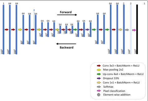
The first CNN architecture proposed in this study for breast lesion semantic segmentation in US image, CNN1, is a series architecture. In this architecture, the input of each layer is the output of the previous layer. A series architec-ture is always used in the studies of Roth et al. [18], the Pure CNN architecture, used for pancreas segmentation in CT images, and Shelhamer et al. [19], the FCN architecture, used for semantic segmentation in general. Figure2shows the proposed CNN1 architecture, obtained empirically through several experiments. We tried smaller architec-tures, but noticed the presence of some noise in the final image. The proposed architecture minimized the presence of noise in the final image. The following layer names are used to describe the network architecture: Convolutional (Conv), Batch Normalization (BatchNorm), Rectifier Linear Unit (ReLU), Maximum Pooling (MaxPooling), Deconvolu-tion (Deconv). The overall net is formed by: (Conv64-BatchNorm-ReLU (2x) – MaxPooling) (3x) – Conv64-BatchNorm-ReLU(2x)– Deconv64-BatchNorm-ReLU- Conv64-BatchNorm-ReLU-Dropout-(Deconv64-Batch-Norm-ReLU-Conv64-BatchNorm-ReLU) (2x)- MaxPool-ing- Conv2-BatchNorm-ReLU-Softmax–PixelClassification. Layers play two important roles with respect to the network operation as a whole: a forward pass that takes the inputs and calculates the outputs, and a backward pass that computes the gradients and adjusts the layer parameters in accordance with them. In the adopted deep learning frame-work, data input is regarded as a layer. In our case, the data type of input layer was the Matlab Image Datastore object, which manages a collection of image files, where each indi-vidual image fits in the memory, but the entire collection of images does not necessarily fit. The network contains

(4)

eleven convolutional layers. The receptive fields of the first ten equal to 3 × 3 pixels and of the last one is 1 × 1 pixel; both padding and stride hyper-parameters are equal to one. All convolutional layers, except the last one, have 64 feature maps. The last convolutional layer produces two feature maps, since pixels will be classified in two classes: (0) back-ground, (1) lesion. All weights of the convolution layers were initialized according to a Gaussian distribution with mean 0 and standard deviation of 0.01. The biases were ini-tialized as constants, with zero as default value. During training, the weights of these convolutional layers are ad-justed to identify visual features, such as edges, orientations or certain patterns in the images. Each convolutional layer is followed by a ReLU layer, which applies an activation function to neurons defined as f(x) = max (0, x), where x is a single neuron input. According to Krizhevsky et al. [20], the ReLU units accelerate network convergence. MaxPool-ing layers progressively reduce the input spatial size to re-duce the number of parameters and computation in the network. All these MaxPooling layers have 2 × 2-sized fil-ters applied with a stride of 2 and padding of 0, down sampling every depth slice in the input by 2 along both width and height, discarding 75% of the activations. The MAX operations take the maximum value from a 2 ×

2-pixel region. The depth dimension remains unchanged. The Dropout layer reduces overfitting by preventing com-plex co-adaptations in training data. A Dropout ratio par-ameter sets the probability that any given unit is dropped. In this work, the dropout ratio parameter was set to 0.5. To speed up training of convolutional neural networks and reduce the sensitivity to network initialization, a Batch Normalization layer is used between convolutional layers and nonlinearities, such as ReLU layers. It normalizes each input channel across a mini-batch. The Deconvolution layers perform an up-sampling to obtain a predictive map of pixel classification with the same size as the input; in other words, it predicts the class to which each pixel belongs. All the Deconvolution layers use filters with receptive fields of 4 × 4 pixels. It works inversely to the convolutional layer. It reuses the convolution layer param-eters, but in the opposite direction, that is, the padding is removed from the output rather than added to the input, and the stride results in an up-sampling rather than a sub-sampling.

The Softmax layer calculates both the softmax and the multinomial logistic loss operations, which saves time and improves numerical stability. It takes two inputs, the first one being the prediction of the prior layer (Conv2) and

(5)

the second one being the label layer. It computes the loss function value, which is used by a backpropagation algo-rithm to calculate the gradients with respect to all weights in the network.

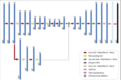
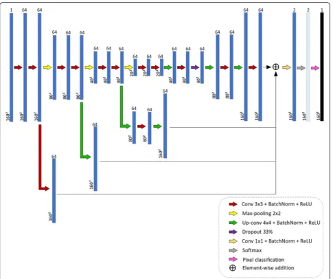
The second and third CNN architectures proposed in this study for breast lesion segmentation in US image, CNN2 and CNN3, are DAG architectures. A DAG archi-tecture has layers arranged as a directed acyclic graph. A DAG architecture is more complex than a series architec-ture, in which layers have inputs from multiple layers and outputs to multiple layers. When applied to image pro-cessing, these architectures aggregate information of pixel localization contained in initial layers into final layers. In semantic tasks, it is expected that this procedure enhances fine image details. The study of Chen et al. [21] used a DAG architecture to segment neuronal structures in Elec-tron Microscope Images. Figures 3 and 4 show the two proposed DAG architectures. In both, the main network path is like CNN1.

In CNN2, information from the first sub-sampling mod-ule, after the second convolution operation, is aggregated before the convolution operation of the first up-sampling module. To implement aggregation, it is necessary that the data representation in both inputs be of the same size.

Since the data dimension after the two convolution opera-tions of the first sub-sampling module is 160 × 160, and after the deconvolution of the first up-sampling module is 40 × 40, a dimension reduction of the first one is neces-sary. This is accomplished with two MaxPooling opera-tions with 2 × 2-sized filters.

In CNN3, information from the three sub-sampling modules, after the second convolution layer of each one, is aggregated before the last convolution layer, Conv2. The number of layers of CNN1, CNN2 and CNN3 is 52, 61 and 68, respectively.

We evaluated the performance of the proposed architec-tures applying various hyper parameter adjustments. For CNN training, the algorithm Stochastic Gradient Descent with Momentum (SGDM) was used. The SGDM algorithm might oscillate along the path of the steepest descent to-wards the optimum. Adding a momentum term to the par-ameter update is one way to reduce this oscillation [22]. The stochastic gradient descent with momentum update is.

θlþ1¼θl−∇Eð Þ þθl γ θð l−θl−1Þ ð1Þ

The momentum γ determines the contribution of the previous gradient step to the current iteration. θ is the

(6)

learning rate and ∇E its gradient. The initial learning rate was set in 0.001 and the momentum in 0.9. Due to limitations in the Graphical Processor Unit memory, batch size was set to 5. Stop condition was set in 150 epochs. This maximum was selected observing the con-vergence of the CNN training.

A quantitative analysis of the performance of the three architectures is made using the following metrics: accur-acy, global accuraccur-acy, IoU, Boundary F1 (BF) score and Dice Similarity Coefficient. The accuracy refers to pro-portion of pixels corrected classified per class, lesion or background, while the global accuracy refers to propor-tion of pixels corrected classified, regardless their class, lesion or background.

Training, validation and testing

Both databases were divided into three subsets: training, validation and testing. In each database, 60% of the data

was used for training, 20% for validation, and 20% for testing. For dataset A, this corresponds to 233, 77, and 77 images. For dataset B, this corresponds to 97, 33, and 33 images. The proportion of malignant and benign lesions in each subset reflected this same proportion. The valid-ation step was used for selecting the CNN architecture with best performance. After choosing the architecture with the best performance in the validation set, the train-ing and test set were merged, and a 5 cross-validation strategy was applied to evaluate it.

Evaluation metrics

The following evaluation metrics were used: global accur-acy, IoU, Dice coefficient and BF score. In the description of these evaluation metrics, we will use the following defi-nitions: False Positives: pixels that belong to the back-ground that were misclassified as belonging to lesions; False Negatives (FN): pixels that belong to lesions that

(7)

were misclassified as belonging to the background; True Positive: pixels that belong to lesions that were correctly classified as belonging to lesions; True Negative (TN): pixels that belong to the background that were correctly classified as belonging to the background.

The global accuracy is the ratio between the pixels correctly classified, regardless of class, and the total number of pixels and is given in Eq. (2):

global accuracy¼ TPþTN

TPþTNþFPþFN ð2Þ

The accuracy gives the proportion of corrected classi-fied pixels in each class and is given in Eq. (3):

accuracy¼ðTP=TPþFNÞ þðTN=TNþFPÞ

2 ð3Þ

The IoU is a metric that penalizes the incorrect classifica-tion of pixels as lesions (FP) or as background (FN), and is given in Eq. (4):

IoU¼LesionþBackground

2 ð4Þ

Where:

Lesion¼ TP

TPþFNþFP ð5Þ

(8)

Background¼ TN

TNþFNþFP ð6Þ

The Weighted IoU is used when there is a dispropor-tionate relation between the class sizes in the images, minimizing the penalty of wrong classifications in smaller classes. It is given in Eq. (7).

Weighted IoU¼Lesion weight x lesion

þBackground weight x background

ð7Þ

Where:

Lesion weight¼number of pixels belonging to lesion total number of pixels

ð8Þ

Brakground weight¼number of pixels belonging to lesion total number of pixels

ð9Þ

The Dice coefficient measures the proportion of pixels correctly classified as lesion, penalizing the incorrect classification (FP or FN), and is given in Eq. (10).

Dice¼ 2TP

2TPþFNþFP ð10Þ

The BF Score measures the alignment between the predicted borders and the gold standard one. It is given

by a weighted harmonic mean of precision and recall, as shown in Eq. (11):

BF score¼2x precisionð þrecallÞ

precisionþrecall ð11Þ

Results

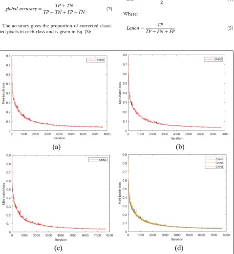
Figure 5 shows the graphs of network convergence, using dataset A, with the SGDM optimization algorithm. In thexandyaxes are the iterations and mini-batch loss values, respectively. During the training, the network weights are adjusted in order to decrease the mini-batch loss value, forcing the algorithm convergence to the minimum. As this is a stochastic process and the weight are randomly initialized, successive trainings on the same dataset do not result in equal weights at the end. As shown in Fig. 5d, the speed convergences of CNN1, CNN2 and CNN3 are almost the same. In these net-works, a plateau is reached after 7000 iterations. With dataset A, the training times of CNN1, CNN2, CNN3 were 95′14″, 112′4″, 183′ 35″, respectively. These training times maintain a strong relationship with the CNN architecture sizes.

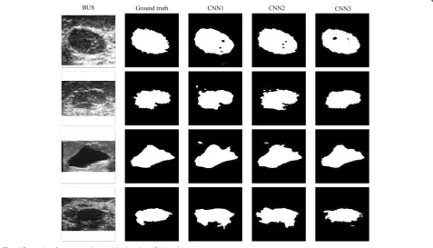
Aiming at a qualitative analysis, Fig.6shows examples of segmentations performed by the three architectures in 3 breast lesions of dataset A. As observed, the contours obtained by CNN1 are smoother than the contours ob-tained by the DAG architectures. The architecture

(9)

CNN1 sub-samples the input image with dimension of 160 × 160 pixels to 20 × 20 pixels and then up-samples to 160 × 160 in the final layers. In this process details of the lesion contours are lost, generating smooth contours such as those shown in Fig. 6. The contours obtained with the DAG architectures, CNN2 and CNN3 have more details and irregularities, like the gold-standard contours. The reason is that these architectures aggre-gate to the last layers information from initial layers, thus preserving pixel localization in the original image.

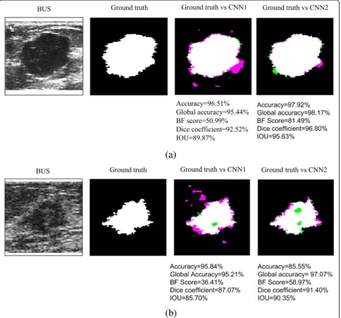
Figure 7a and b show a quantitative analysis of a be-nign and a malignant lesion, respectively, obtained from dataset A. The pink color shows false positive pixels

(pixels outside the ground truth contour considered as inside, in the obtained contour), while green color shows false negative pixels. The contour with lower number of false positives and false negatives pixels is the one ob-tained with CNN3. Below each image the metrics of each contour are shown. As can be seen, the best met-rics values are also obtained with CNN3.

Tables1 and 2show the results of the validation step, for datasets A and B. The best values are shown in boldface.

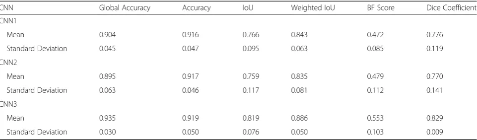
Comparing Tables 1 and 2, we notice that CNN3 presents the best values for all metrics and for both da-tabases. The best values of global accuracy, mean

(10)

accuracy, weighted IoU and mean BF score were ob-tained with dataset A, while the best values for mean IoU and Dice coefficient were obtained with dataset B.

The differences between the global accuracies in each dataset were evaluated using t-student hypothesis test. The calculated value oft-studenttest is compared with a critical valuetc. The null hypothesis is rejected if or t≥ tc or t≤ −tc. In the first case, the mean value is

consid-ered significantly higher, and, in the second case, signifi-cantly lower. In this study, a confidence level of 95%, 152 degrees of freedom were used for dataset A, corre-sponding to a critical value of tc= 1.982. For dataset B

we have 64 degrees of freedom, corresponding to a crit-ical value oftc= 2.000.

Comparing the results of CNN3 with CNN2 in dataset A, we obtained a t-value =5.062. This value is statisti-cally significant. Comparing the results of CNN2 with CNN1 in dataset A, we obtained at-value=−1.026, not statistically significant. Comparing the results of CNN3 with CNN1 in dataset A, we obtained a t-value=5.062. This result is statistically significant. Comparing the re-sults of CNN3 with CNN2 in dataset B, we obtained a t-value =1.078. This result is not statistically significant.

Comparing the results of CNN2 with CNN1 in dataset A we obtained at-value=−0.605. This result is not sta-tistically significant. Comparing the results of CNN3 with CNN1 in dataset A, we obtained a t-value=0.381. This result is not statistically significant.

Therefore, although the best metrics values are ob-tained with CNN3, the differences in Global Accuracies obtained with this network and with CNN2 and CNN1 are statistically significant only for dataset A.

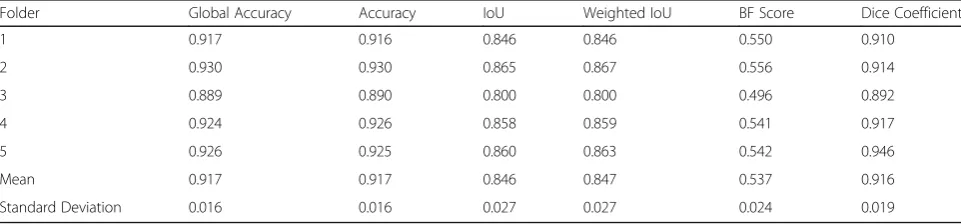
Tables 3 and 4 shows results using CNN3 and cross-validation with 5 folders, for datasets A and B, respectively. The networks were trained and tested with cropped images resized to 160 × 160 pixels. Comparing Tables3and4, we notice that the best values of all metrics were obtained with dataset A. The differences between the global accuracies were evaluated usingt-student hypothesis test. The calcu-lated value oft-studenttest is compared with a critical value

tc. In this study, a confidence level of 99% and 5 degrees of

freedom were used (5 folders), corresponding to a critical value oftc= 4.032. We obtained at-value=4.183. This value

is statistically significant.

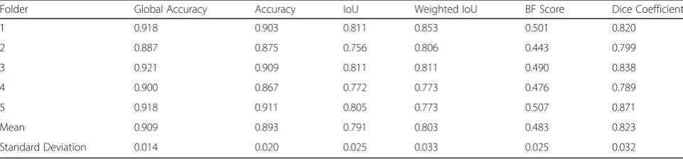
Tables 5 and 6 shows the results obtained using CNN3 and cross validation with 5 folders, for dataset

Table 2Mean values of the metrics for the dataset B, using the validation set and cropped images resized to 160 × 160 pixels

CNN Global Accuracy Accuracy IoU Weighted IoU BF Score Dice Coefficient

CNN1

Mean 0.917 0.904 0.836 0.850 0.510 0.920

Standard Deviation 0.048 0.068 0.090 0.079 0.083 0.032

CNN2

Mean 0.911 0.895 0.823 0.838 0.515 0.915

CNN3

Mean 0.921 0.914 0.845 0.857 0.516 0.918

Table 1Mean values of the metrics for the dataset A, using the validation set and cropped images resized to 160 × 160 pixels

CNN Global Accuracy Accuracy IoU Weighted IoU BF Score Dice Coefficient

CNN1

Mean 0.904 0.916 0.766 0.843 0.472 0.776

CNN2

Mean 0.895 0.917 0.759 0.835 0.479 0.770

CNN3

Mean 0.935 0.919 0.819 0.886 0.553 0.829

(11)

B, with original images resized to 160 × 160 pixels and 320 × 320 pixels.

Comparing Tables 4 and 5, we notice that the best values of mean accuracy, mean IoU and Dice coeffi-cient were obtained with dataset B with cropped im-ages resized to 160 × 160 pixels, while the best values for global accuracy, weighted IoU and mean BF score were obtained with dataset B, with original images resized to 160 × 160 pixels. The differences between the global accuracies were evaluated using t-student

hypothesis test. The calculated value of t-student test is compared with a critical value tc. In this study, a

confidence level of 95% and 8 degrees of freedom were used, corresponding to a critical value of tc=

3.355. We obtained a t-value =−7.938. This value is statistically significant.

Comparing Tables 5 and 6, we notice that the best values of global accuracy, mean IoU, weighted IoU and mean BF score were obtained with dataset B, with ori-ginal images resized to 160 × 160 pixels, whereas the best values for Mean Accuracy and Dice Coefficient were ob-tained with dataset B, with original images resized to 320 × 320 pixels. The differences between the global ac-curacies were evaluated using t-student hypothesis test. The calculated value oft-studenttest is compared with a critical value tc. In this study, a confidence level of 95%

and 8 degrees of freedom were used, corresponding to a critical value of tc= 3.355. We obtained a t-value =

10.000. This value is statistically significant.

Discussion

The main advantage of CNNs compared with trad-itional machine learning techniques in segmentation and classification tasks, is that the former are fully automated, requiring no pre-processing for character-istic extraction.

The performance of CNNs is strongly dependent on the existence of large databases. This is a challenge for medical applications, since we have relatively small datasets in this research area. In previous studies pub-lished in the literature for breast lesion segmentation, it was shown (digital mammography [11–13] and US [10]) that, even with small datasets, CNN outperforms the traditional machine learning techniques in breast lesion segmentation and classification. Dataset A used in this study comprises 387 US images: 208 are benign lesions and 179 are malignant lesions. Compared with other datasets previously cited and used for breast le-sion segmentation, 50 images [5], 112 images [6] and 30 images [8], dataset A is the larger one.

In deep learning, there is a plenty of CNN architec-tures that have been proposed for image segmentation and classification. It is impossible to evaluate all these architectures in each application. From previous knowledge of the characteristics of each architecture, it is possible to select an appropriate one, with tailored characteristics to solve a given problem.

In this study, the main task was to evaluate if CNN architectures could outline irregular contours, with

Table 4Metrics values for cross-validation with 5 folders for dataset B, using cropped images resized for 160 × 160 pixels

Folder Global Accuracy Accuracy IoU Weighted IoU BF Score Dice Coefficient

1 0.917 0.916 0.846 0.846 0.550 0.910

2 0.930 0.930 0.865 0.867 0.556 0.914

3 0.889 0.890 0.800 0.800 0.496 0.892

4 0.924 0.926 0.858 0.859 0.541 0.917

5 0.926 0.925 0.860 0.863 0.542 0.946

Mean 0.917 0.917 0.846 0.847 0.537 0.916

Table 3Metrics values for cross-validation with 5 folders for dataset A, using cropped images resized for 160 × 160 pixels

1 0.952 0.944 0.864 0.913 0.679 0.877

2 0.969 0.961 0.904 0.942 0.754 0.916

3 0.936 0.944 0.834 0.887 0.603 0.850

4 0.961 0.947 0.884 0.923 0.704 0.904

5 0.964 0.954 0.894 0.932 0.724 0.915

Mean 0.956 0.950 0.876 0.920 0.693 0.918

(12)

spiculation and angulated margins, such as those found in US breast lesions images. Our choice was to use DAG architectures. From a previous knowledge of the performance of the DAG architecture in image segmentation applications, we knew that these archi-tectures aggregate information of pixel localization contained in initial layers into final layers, preserving fine image details. In this study, the performance of the DAG architectures, compared with a series archi-tecture, is superior, both qualitatively as quantitatively.

The comparison of the performance of CNN3, CNN2 and CNN1 in Tables 1and 2 shows that CNN3 present best performance for all metrics in both datasets. How-ever, the differences between global accuracies are only statistically significant in dataset A.

The comparison of the metrics in Tables 3 and 4, where cropped images resized to 160 × 160 are used, shows that all the best metrics values are obtained with dataset A. The differences between the obtained global accuracies are statistically significant. As stated by Yap et al. [10], we believe that high quality images (dataset B) may include other structures such as ribs, pectoral muscle or air in the lungs, making the lesion segmenta-tion more difficult.

In Tables 4, 5, and 6 we also compared three varia-tions of database B: one with cropped images resized to 160 × 160, another with original images resized to 160 × 160 pixels and another with original images resized to 320 × 320 pixels. The comparison showed that some metrics were higher in some than others. However, the

global accuracy obtained with original images resized to 160 × 160 pixels is better than those obtained with the other two image sets, and the differences are statistically significant.

Comparing this study with other studies using conven-tional machine learning techniques we noticed that: Infantosi et al. [16], using a subset of dataset A, com-posed of 200 images, doing the lesion segmentation with morphologic operators and a gaussian function con-straint, observed that 91% of the images presented an IoU better than 0.5. Gomez et al. [17] using a subset of dataset A, composed of 50 images, doing the lesion seg-mentation using marker-controlled watershed trans-formation, obtained an IoU value of 0.86 ± 0.05. In this study, with CNN3 and dataset A, we obtained a mean IoU of 0.876 and a weighted IoU of 0.920; Jiang et al. [7], as previously cited, obtained an Accuracy of 87.5% using a different dataset. In this study, with CNN3 and dataset A, we obtained an accuracy of 0.950 ± 0.006 and a global accuracy of 0.956 ± 0.011. Torbati et al. [8], as previously cited, obtained an IoU of 86.95% using a data-set with 30 images.

Conclusion

In this study we evaluated the performance of CNN ar-chitectures in the task of breast lesion segmentation in US images. Our main concern was to assess the ability of CNNs to detect contour irregularities in breast lesions in US images.

Table 6Metrics values for cross-validation with 5 folders for dataset B, using original images resized for 320 × 320 pixels

1 0.918 0.903 0.811 0.853 0.501 0.820

2 0.887 0.875 0.756 0.806 0.443 0.799

3 0.921 0.909 0.811 0.811 0.490 0.838

4 0.900 0.867 0.772 0.773 0.476 0.789

5 0.918 0.911 0.805 0.773 0.507 0.871

Mean 0.909 0.893 0.791 0.803 0.483 0.823

Table 5Metrics values for cross-validation with 5 folders, for dataset B, using original images resized for 160 × 160 pixels

1 0.982 0.915 0.806 0.969 0.669 0.692

2 0.987 0.900 0.844 0.976 0.730 0.758

3 0.977 0.833 0.744 0.960 0.597 0.574

4 0.970 0.820 0.738 0.947 0.630 0.608

5 0.983 0.933 0.837 0.969 0.693 0.714

Mean 0.979 0.880 0.794 0.964 0.664 0.669

(13)

A qualitative analysis showed that DAG architec-tures better represent the irregularities present in the gold-standard contours traced by a specialist. The best results were obtained with the more complex DAG architecture.

As future work, we propose evaluating DAG architec-tures in a large database, which would enable a better network generalization.

Abbreviations

BatchNorm:Batch Normalization; BF: Boundary F1; BUS: Breast Ultrasound Images; CAD: Computer-Aided Diagnosis; CNN: Convolutional Neural Network; Conv: Convolutional; CPU: Central Processor Unit; DAG: Direct Acyclic Graph; Deconv: Deconvolutional; DM: Digital mammography; FCN: Fully Convolutional Network; FN: False Negatives; FP: False Positives; GB: Giga Bytes; IoU: Intersection over Union; MaxPooling: Maximum Pooling; RAM: Random Access Memory; ReLU: Rectifier Linear Unit; SGDM: Stochastic Gradient Descent with Momentum; TN: True Negatives; TP: True Positives; US: Ultrasound

Acknowledgements

Academic English Solutions (https://www.academicenglishsolutions.com) revised this paper.

Authors’contributions

Conception and design of the work: MGFC, JPMC, GAA and CFFCF. data collection: WCAP. Drafting the article: CFFCF. Final approval of the article: MGFC. All authors read and approved the final manuscript.

Funding

This research, according for in Article 48 of Decree n° 6.008/2006, was funded by Samsung Electronics of Amazonia Ltda, under the terms of Federal Law n° 8.387/1991, through agreement n° 004, signed with the Center for R&D in Electronics and Information from the Federal University of Amazonas - CETELI/UFAM; Coordenação de Aperfeiçoamento de Pessoal de Nível Superior–Brasil (CAPES)–Funding Code 001, and Fundação de Amparo a Pesquisa do Estado do Amazonas (FAPEAM), process #062.00575/ 2014-PROTI-PESQUISA and process #062.00710/2016–PAPAC. Academic English Solutions (https://www.academicenglishsolutions.com) revised this paper.

Availability of data and materials

The data that support this study will be provided upon request to the authors, only for academic research purposes and with the commitment to cite this work.

Ethics approval and consent to participate

National Cancer Institute (INCa) Ethics Committee, of Rio de Janeiro, Brazil, has approved this study (38/2001).

Consent for publication

Not applicable.

Competing interests

The authors declare that they have no competing interests.

Author details

1_{Centro de Tecnologia Eletrônica e da Informação/Universidade Federal do}

Amazonas, Av. General Rodrigo Otávio Jordão Ramos, 3000, Aleixo, Campus Universitário–Setor Norte, Pavilhão Ceteli, Manaus, AM CEP: 69077-000, Brazil.2_{Programa de Engenharia Biomédica/COPPE/Universidade Federal do}

Rio de Janeiro, Rio de Janeiro, Brazil.

Received: 6 March 2019 Accepted: 16 October 2019

References

1. Siegel RL, Miller KD, Jemal A. Cancer statics 2017. CA Cancer J Clin. 2017; 67(1):7–30.

2. Stewart BW, Wild CP. World cancer report 2018: World Health Organization; 2018. Edited by, WHO.https://www.who.int/cancer/PRGlobocanFinal.pdf. Accessed 23 Aug 2019

3. Akin O, Brennan S, Dershaw D, Ginsberg M, Gollub M, Schoder H, Panicek D, Hricak H. Advances in oncologic imaging: update on 5 common cancers. CA Cancer J Clin. 2012;62(6):364_–93.

4. Stavros A, Thickman D, Rapp C, Dennis M, Parker S, Sisney G. Solid breast nodules: use of sonography to distinguish between benign and malignant lesions. Radiology. 1995;196(1):123–34.

5. Daoud MI, Atallah AA, Awwad F, Al-Najar M. Accurate and fully automatic segmentation of breast ultrasound images by combining image boundary and region information. In: International Symposium on Biomedical Imaging; 2016. p. 718–21.

6. Liu L, Qin W, Yang R, Yu C, Li L, Wen T, Gu J. Segmentation of breast ultrasound image using graph cuts and level set. In: Int. Conf. on Biom. Image and Signal Proces; 2015. p. 1–4.

7. Jiang P, Peng J, Zhang G, Cheng E, Megalooikonomou V, Ling H. Learning-based automatic breast tumor detection and segmentation in ultrasound images. In: IEEE Int. Symp. on Biom. Imaging; 2012. p. 1587–90.

8. Torbati N, Ayatollahi A, Kermani A. Ultrasound image segmentation by using a FIR neural network. In: Iranian Conf. on Electrical Engineering; 2013. p. 1_–5.

9. Zhao F, Li X, Biswas S, Mullick R, Mendonça PRS, Vaidya V. Topological texture-based method for mass detection in breast ultrasound image. In: Int. Symp. on Biom. Imaging; 2014. p. 685–9.

10. Yap MH, Pons G, Martí J, Ganau S, Sentís M, Zwiggelaar R, Davison AK, Martí R. Automated breast ultrasound lesions detection using convolutional neural networks. IEEE J Biomed Health Inform. 2017;22(4):1218–26. 11. Dhungel N, Carneiro G, Bradley AP. Deep learning and structured prediction

for the segmentation of mass in mammograms. In: Proc. Int. Conf. Med. Image Comput. Comput.-Assisted Intervention; 2015. p. 605–12. 12. Mordang JJ, Janssen T, Bria A, Kooi T, Gubern-Merida A, Karssemeijer N.

Automatic microcalcification detection in multi-vendor mammography using convolutional neural networks. In: Proc. Int. Workshop Digital Mammography; 2016. p. 35–42.

13. Ahn CK, Heo C, Jin H, Kim JH. A novel deep learning-based approach to high accuracy breast density estimation in digital mammography. In: Proc. SPIE, vol. 10134; 2017. p. 101 342O.

14. Long J, Shelhamer E, Darrell T. Fully convolutional networks for semantic segmentation. In: Proc. IEEE Conf. Comput. Vis. Pattern Recognit; 2015. p. 3431–40.

15. Ronneberger O, Fischer P, Brox T. U-net: convolutional networks for biomedical image segmentation. In: International conference on medical image computing and computer-assisted intervention; 2015. p. 234–41. 16. Infantosi AFC, Pereira WCA, Luz LMS, Alvarenga AV. Breast ultrasound

segmentation using morphologic operators and a Gaussian function constraint. In: 14th Nordic-Baltic conference on biomedical engineering and medical physics; 2008. p. 520–3.

17. Gomez W, Leija L, Alvarenga AV, Infantosi AFC, Pereira WCA. Computerized lesion segmentation of breast ultrasound based on marker-controlled watershed transformation. Med Phys. 2010;37(1):82–95.

18. Roth HR, Farag A, Lu L, Turkbey EB, Summers RM. Deep convolutional networks for pancreas segmentation in CT imaging. Ourselin, Sébastien and Styner, Martin A. Editors. Medical Imaging: Image Processing. SPIE; 2015. p. 94131G–94131G-8.http://dx.doi.org/10.1117/12.2081420.

19. Shelhamer E, Long J, Darrell T. Fully convolutional networks for semantic segmentation. IEEE Trans Pattern Anal Mach Intell. 2017;39(4):640–51. 20. Krizhevsky A, Sutskever I, Hinton G. ImageNet classification with deep

convolutional neural networks. Adv Neural Inf Process Syst. 2012;25:1106–14. 21. Chen H, Qi XJ, Cheng JZ, Heng PA. Deep contextual networks for neuronal

structure segmentation. In: Thirtieth AAAI conference on artificial intelligence; 2016. p. 1167_–73.

22. Goodfellow I, Bengio Y, Courville A. Deep Learning: MIT Press; 2016. ISBN 9780262035613. Accessed inhttps://books.google.com.br/books?id= Np9SDQAAQBAJ

Publisher’s Note