Cognitive Sciences EPrint Archive (CogPrints) 7056, (2010) http://cogprints.org/7056/
An Extension of Slow Feature Analysis for
Nonlinear Blind Source Separation
Henning Sprekeler
∗(
[email protected]
)
Tiziano Zito (
[email protected]
)
and Laurenz Wiskott (
[email protected]
)
Institute for Theoretical Biology
& Bernstein Center for Computational Neuroscience Berlin
Humboldt University Berlin
Unter den Linden 6
10099 Berlin, Germany
We present and test an extension of slow feature analysis as a novel approach to nonlinear blind source separation. The algorithm relies on temporal correlations and iteratively reconstructs a set of statistically independent sources from arbitrary nonlinear instantaneous mixtures. Simulations show that it is able to invert a complicated nonlinear mix-ture of two audio signals with a reliability of more than 90%. The algorithm is based on a mathematical analysis of slow feature analysis for the case of input data that are generated from statistically inde-pendent sources.
1 Introduction
Independent Component Analysis (ICA) as a technique for blind source separation (BSS) has attracted a fair amount of research activity over the past two decades. By now a number of techniques have been established that reliably reconstruct the underlying sources from linear mixtures (Hyv¨arinen et al., 2001). The key insight for linear BSS is that the statistical independence of the sources is usually sufficient to constrain the unmixing function up to trivial transformations like permutation and scaling. Therefore linear BSS is essentially equivalent to linear ICA.
An obvious extension of the linear case is the task of reconstructing the sources from nonlinear mixtures. Unfortunately, the problem of nonlinear BSS is much harder than linear BSS, mainly due to the fact that the statistical independence of the instantaneous values of the estimated sources is no longer a sufficient constraint for the unmixing (Hyv¨arinen and Pajunen, 1999). For example, arbitrary point-nonlinear distortions of the sources are still statistically independent. Therefore, additional constraints are needed to resolve these ambiguities.
c
2010 Sprekeler, Zito, Wiskott
∗corresponding author; now at: Laboratory for Computational Neuroscience, ´Ecole
One approach is to exploit the temporal structure of the sources (e.g., Harmel-ing et al., 2003; Blaschke et al., 2007). Blaschke et al. (2007) proposed to use the tendency of nonlinearly distorted versions of the sources to vary more quickly in time than the original sources. A simple illustration for this effect is the frequency doubling property of a quadratic nonlinearity when applied to a sine wave. This observation opens the possibility of finding the original source (or a good repre-sentative thereof) among all the nonlinearly distorted versions by choosing the one that varies most slowly in time. An algorithm that has been specifically designed for extracting slowly varying signals is Slow Feature Analysis (SFA, Wiskott, 1998; Wiskott and Sejnowski, 2002). Moreover, SFA is intimately related to ICA tech-niques like TDSEP (Ziehe and M¨uller, 1998; Blaschke et al., 2006) and differential decorrelation (Choi, 2006) and is therefore an interesting starting point for devel-oping nonlinear BSS techniques.
Here, we extend a previously developed mathematical analysis of SFA (Franzius et al., 2007) to the case where the input data are generated from a set of statistically independent sources. The theory makes clear predictions as to how the sources are represented by the output signals of SFA. Based on these predictions, we develop a new algorithm for nonlinear blind source separation. Because the algorithm is an extension of SFA, we refer to it as xSFA.
The structure of the paper is as follows. In section 2, we introduce the opti-mization problem for SFA and give a brief sketch of the SFA algorithm. In Section 3 we develop the theory that underlies the xSFA algorithm. In section 4, we present the xSFA algorithm and evaluate its performance on nonlinear mixtures of audio signals. Limitations and possible reasons for failures are discussed in section 5. We conclude with a general discussion in section 6.
2 Slow Feature Analysis
In this section, we briefly present the optimization problem that underlies slow feature analysis and sketch the algorithm that solves it.
2.1 The Optimization Problem
Slow Feature Analysis is based on the following optimization task: For a given multi-dimensional input signal we want to find a set of scalar functions that gen-erate output signals that vary as slowly as possible. To ensure that these signals carry significant information about the input, we require them to be uncorrelated and have zero mean and unit variance. Mathematically, this can be stated as fol-lows:
Optimization problem 1: Given a function space F and an N-dimensional input signal x(t) find a set ofJ real-valued input-output functionsgj(x)∈ F such
that the output signals yj(t) :=gj(x(t))minimize
∆(yj) =hy˙2jit (1)
under the constraints
hyjit = 0 (zero mean), (2)
hyj2it = 1 (unit variance), (3)
∀i < j:hyiyjit = 0 (decorrelation and order), (4)
withh·it andy˙ indicating temporal averaging and the derivative ofy, respectively.
decorrelation constraint (4) forces different functionsgjto encode different aspects
of the input. Note that the decorrelation constraint is asymmetric: The function
g1 is the slowest function inF, while the functiong2 is the slowest function that fulfills the constraint of generating a signal that is uncorrelated to the output sig-nal ofg1. The resulting sequence of functions is therefore ordered according to the slowness of their output signals on the training data.
It is important to note that although the objective is the slowness of the output signal, the functionsgjare instantaneous functions of the input, so that slowness
cannot be achieved by low-pass filtering. As a side effect, this makes SFA unsuit-able for inverting convolutive mixtures.
2.2 The SFA Algorithm
IfF is finite-dimensional, the problem can be solved efficiently by the SFA algo-rithm (Wiskott and Sejnowski, 2002; Berkes and Wiskott, 2005). The full algoalgo-rithm can be split in two parts: a nonlinear expansion of the input data, followed by a linear generalized eigenvalue problem.
For the nonlinear expansion, we choose a set of functionsfi(x) that form a basis
of the function spaceF. The optimal functionsgjcan then be expressed as linear
combinations of these basis functions: gj(x) =PiWjifi(x). By applying the basis
functions to the input datax(t), we get a new and generally high-dimensional set of signalszi(t) =fi(x(t)). Without loss of generality, we assume that the functions
fi are chosen such that the expanded signalszi have zero mean. Otherwise, this
can be achieved easily by subtracting the mean.
After the nonlinear expansion, the coefficients Wji for the optimal functions
can be found from a generalized eigenvalue problem:
˙
CW=CWΛ. (5)
Here, ˙Cis the matrix of the second moments of the temporal derivative ˙ziof the
expanded signals: ˙Cij=hz˙i(t) ˙zj(t)it. Cis the covariance matrixC=hzi(t)zj(t)it
of the expanded signals (sincezhas zero mean),Wis a matrix that contains the weightsWjifor the optimal functions andΛis a diagonal matrix which contains
the generalized eigenvalues on the diagonal.
If the function spaceF is the set of linear functions, the algorithm reduces to solving the generalized eigenvalue problem (5). Therefore, the second step of the algorithm is in the following referred to as linear SFA.
3 Theoretical Foundations
In this section we extend previous analytical results for SFA to the case of nonlinear blind source separation, more precisely, to the case where the input datax(t) are generated from a set of statistically independent sourcess(t) by means of a nonlin-ear, instantaneous, and invertible (or at least injective) function: x(t) =F(s(t)). For readers that are more interested in the algorithm than in its mathematical foundations, a summary of the relevant theoretical results can be found at the end of the section.
3.1 SFA with Unrestricted Function Spaces
Conceptual Consequences of an Unrestricted Function Space
The central assumption for the theory is that the function spaceF that SFA can access is unrestricted. This has important conceptual consequences.
generates an output signaly(t) =g(x(t)) when applied to the mixturex(t). Then, for every such function g, there is another function ˜g=g◦Fthat generates the same output signal y(t) when applied to the sources s(t) directly. Because the function spaceF is unrestricted, this function ˜gis also an element of the function spaceF. Because this is true for all functionsg∈ F, the set of output signals that can be generated by applying the functions in F to the mixturex(t) is the same as the set of output signals that can be generated by applying the functions to the sourcess(t) directly. Because the optimization problem of SFA is formulated purely in terms of output signals, the output signals when applying SFA to the mixture are the same as when applied directly to the sources. In other words: For an unrestricted function space, the output signals of SFA are independent of the structure of the mixing functionF. This statement can be generalized to the case where the mixturex has a higher dimensionality than the sources, as long as the mixing functionFis injective.
Given that the output signals are independent of the mixture, we can make analytical predictions about the dependence of the output signals on the sources, when the input signals are not a mixture, but the sources themselves. The results of such an analysis generalize to the case where the input signals are a nonlinear mixture of the sources instead.
Of course, an unrestricted function space cannot be implemented in practise. Therefore, in any application the output signals will depend on the mixture and on the function space used. Nevertheless, the idealized case provides important theoretical insights, which we use as the basis for the blind source separation algorithm presented later.
Earlier Results for SFA with an Unrestricted Function Space
In a previous article (Franzius et al., 2007), we have shown that the optimal func-tionsgj(x) for SFA in the case of an unrestricted function space are given by the
solutions of an eigenvalue equation for a partial differential operatorD
Dgj(x) =λjgj(x) (6)
with von Neumann boundary conditions
X
αβ
nαpx(x)Kαβ(x)∂βgj(x) = 0. (7)
Here,Ddenotes the operator
D=− 1
px(x)
X
α,β
∂αpx(x)Kαβ(x)∂β, (8)
px(x) is the probability density of the input dataxand∂α the partial derivative
with respect to theα-th componentxαof the input data. Kαβ(x) =hx˙αx˙βix˙|xis the matrix of the second moments of the velocity distributionp( ˙x|x) of the input data, conditioned on their valuexandnα(x) is theα-th component of the normal
vector on the boundary point x. Note that the partial derivative∂α acts on all
terms to its right, so thatDis a partial differential operator of second order. The optimal functions for SFA are theJ eigenfunctionsgj with the smallest
eigenvaluesλj.
3.2 Factorization of the Optimal Functions
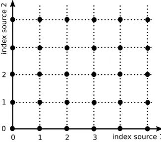
Figure 1:Schematic ordering of the optimal functions for SFA.For an unrestricted function space and statistically independent sources, the optimal functions for SFA are products of harmonics, each of which depends on one of the sources only. In the case of two sources, the optimal functions can therefore be arranged schematically on a 2-dimensional grid, where every grid point represents one function and its coordinates in the grid are the indices of the harmonics that are multiplied to form the function. Because the 0-th harmonic is the constant, the functions on the axes are simply the harmonics themselves and therefore depend on one of the sources only. Moreover, the grid points (1,0) and (0,1) are monotonic functions of the sources and therefore a good representative thereof. It is these solutions that the xSFA algorithm is designed to extract. Note that the scheme also contains an ordering by slowness: All functions to the upper right of a given function have higher ∆-values and therefore vary more quickly.
about their probability distribution and consequently also about the matrixKαβ.
The joint probability density for the sources and their derivatives factorizes:
ps,s(˙ s,s˙) =
Y
α
psα,s˙α(sα,s˙α). (9)
Clearly, the marginal probability densitypsalso factorizes into the individual prob-ability densitiespα(sα)
ps(s) =Y
α
pα(sα), (10)
and the matrix Kαβ of the second moments of the velocity distribution of the
sources is diagonal
Kαβ(s) :=hs˙αs˙βis˙|s=δαβKα(sα) with Kα(sα) :=hs˙2αis˙α|sα. (11)
The latter is true because the mean temporal derivative of 1-dimensional stationary and differentiable stochastic processes vanishes for any sα for continuity reasons,
so thatKαβ is not only the matrix of the second moments of the derivatives, but
actually the conditional covariance matrix of the derivatives of the sources given the sources. As the sources are statistically independent, their derivatives are uncorrelated andKαβ has to be diagonal.
We can now insert the specific form (10,11) of the probability distribution ps and the matrixKαβ into the definition (8) of the operatorD. A brief calculation
shows that this leads to a separation of the operatorDinto a sum of operatorsDα,
each of which depends on only one of the sources:
D(s) =X
α
Dα(sα) (12)
with
Dα=−
1
pα
This has the important implication that the solution to the full eigenvalue prob-lem forDcan be constructed from the 1-dimensional eigenvalue problems for the individual sources:
Theorem 1. Letgαi(i∈N) be the normalized eigenfunctions of the operatorsDα,
i.e., the set of functionsgαi that fulfill the eigenvalue equations
Dαgαi=λαigαi (14)
with the boundary conditions
pαKα∂αgαi= 0 (15)
and the normalization condition
(gαi, gαi)α:=hg2αiisα= 1. (16) Then, the product functions
gi(s) :=Y
α
gαiα(sα) (17)
form a complete set of (normalized) eigenfunctions to the full operatorDwith the eigenvalues
λi=
X
α
λαiα (18)
and thus thosegiwith the smallest eigenvaluesλiare the optimal functions for SFA.
Here,i= (i1, ..., iS)∈NSdenotes a multi-index that enumerates the eigenfunctions of the full eigenvalue problem.
In the following, we assume that the eigenfunctionsgαi are ordered by their
eigenvalue and refer to them as theharmonicsof the sourcesα. This is motivated
by the observation that in the case where pα and Kα are independent of sα,
i.e., for a uniform distribution, the eigenfunctions gαi are harmonic oscillations
whose frequency increases linearly with i(see below). Moreover, we assume that the sources sα are ordered according to slowness, in this case measured by the
eigenvalue λα1 of their lowest non-constant harmonicgα1. These eigenvalues are
the ∆-value of the slowest possible nonlinear point transformations of the sources. The key result of theorem 1 is that in the case of statistically independent sources, the output signals are products of harmonics of the sources. Note that the constant functiongα0(sα) = 1 is an eigenfunction with eigenvalue 0 to all the
eigenvalue problems (14). As a consequence, the harmonicsgαiof the single sources
are also eigenfunctions to the full operator D (with the indexi = (0, ...,0, iα =
i,0, ...,0)) and can thus be found by SFA. Importantly, the lowest non-constant harmonic of the slowest source (i.e., g(1,0,0,...) = g11) is the function with the
smallest overall ∆-value (apart from the constant) and thus the first function found by SFA. In the next sections, we show that the lowest non-constant harmonicsgα1
reconstruct the sources up to a monotonic and thus invertible point transformation and that in the case of sources with Gaussian statistics, they even reproduce the sources exactly.
3.3 The First Harmonic is a Monotonic Function of the Source
The eigenvalue problem (14,15) has the form of a Sturm-Liouville problem (Courant and Hilbert, 1989) and can easily be rewritten to have the standard form for these problems:
∂αpαKα∂αgαi+λαipαgαi
(14,13)
= 0, (19)
with pαKα∂αgαi
(15)
Here, we assume that the sourcesα is bounded and takes on values on the
inter-valsα∈[a, b]. Note that bothpαandpαKαare positive for allsα. Sturm-Liouville
theory states that the solutionsgαi, i∈N0of this problem are oscillatory and that
gαihas exactlyizeros on ]a, b[ if thegαiare ordered by increasing eigenvalueλαi
(Courant and Hilbert, 1989, chapter IV,§6). All eigenvalues are positive. In par-ticular,gα1has only one zeroξ∈]a, b[. Without loss of generality we assume that gα1<0 forsα< ξandgα1>0 forsα> ξ. Then equation (19) implies that
∂αpαKα∂αgα1 =−λαpαgα1<0 forsα> ξ (21)
=⇒ pαKα∂αgα1 is monotonically decreasing on ]ξ, b] (22) (20)
=⇒ pαKα∂αgα1>0 on ]ξ, b[ (23)
=⇒ ∂αgα1>0 since pαKα>0 on ]ξ, b[ (24)
⇐⇒ gα1 is monotonically increasing on ]ξ, b[. (25)
A similar consideration fors < ξ shows thatgα1 is also monotonically increasing
on ]a, ξ[. Thus,gα1 is monotonic and invertible on the whole interval [a, b]. Note
that the monotony ofgα1 is important in the context of blind source separation,
because it ensures that not only some of the output signals of SFA depend on only one of the sources (the harmonics), but that there should actually be some (the lowest non-constant harmonics) that are very similar to the source itself.
3.4 Gaussian Sources
We now consider the situation that the sources are reversible Gaussian stochastic processes, (i.e., that the joint probability density ofs(t) ands(t+dt) is Gaussian and symmetric with respect tos(t) ands(t+dt)). In this case, the instantaneous values of the sources and their temporal derivatives are statistically independent, i.e.,ps˙α|sα( ˙sα|sα) =ps˙α( ˙sα). Thus,Kαis independent ofsα, i.e.,Kα(sα) =Kα=
const. Without loss of generality we assume that the sources have unit variance. Then the probability density of the source is given by
pα(sα) =
1
√
2πe
−s2α/2
(26)
and the eigenvalue equations (19) for the harmonics can be written as
∂αe
−s2α/2 ∂αgαi+
λαi
Kα
e−s2α/2g
αi= 0. (27)
This is a standard form of Hermite’s differential equation (see Courant and Hilbert, 1989, chapter V, §10). Accordingly, the harmonicsgαi are given by the
(appro-priately normalized) Hermite polynomialsHiof the sources:
gαi(sα) =
1
√
2ii!Hi
sα
√
2
. (28)
The Hermite polynomials can be expressed in terms of derivatives of the Gaussian distribution:
Hn(x) = (−1)nex
2
∂xne
−x2
. (29)
It is clear that Hermite polynomials fulfill the boundary condition
lim
sα→∞
Kαpα∂αgαi= 0, (30)
because the derivative of a polynomial is again a polynomial and the Gaussian distribution decays faster than polynomially as|sα| → ∞. The eigenvalues depend
linearly on the indexi:
The most important consequence is that the lowest non-constant harmonics simply reproduce the sources: gα1(sα) = 1/
√
2H1(sα/
√
2) = sα. Thus, for Gaussian
sources, some of the output signals of SFA with an unrestricted function space reproduce the sources exactly.
3.5 Homogeneously Distributed Sources
Another canonical example for which the eigenvalue equation (14) can be solved analytically is the case of homogeneously distributed sources, i.e., the case where the probability distributionps,s˙ is independent of s on a finite interval and zero
elsewhere. Consequently, neitherpα(sα) norKα(sα) can depend onsα, i.e., they
are constants. Note that such a distribution may be difficult to implement by a real differentiable process, because the velocity distribution should be different at boundaries that cannot be crossed. Nevertheless, this case provides an approxi-mation to cases, where the distribution is close to homogeneous.
Letsα take values in the interval [0, Lα]. The eigenvalue equation (19) for the
harmonics is then given by
Kα∂2αgαi+λαigαi= 0 (32)
and readily solved by harmonic oscillations:
gαi(sα) =
√
2 cos
iπsα Lα
. (33)
The ∆-value of these functions is given by
∆(gαi) =λαi=Kα
π Lα
i
2
. (34)
Note the similarity of these solutions with the optimal free responses derived by Wiskott (2003).
3.6 Summary: Results of the Theory
The following key results of the theory form the basis of the xSFA algorithm:
• For an unrestricted function space, the output signals generated by the op-timal functions of SFA are independent of the nonlinear mixture, given the same original sources.
• The optimal functions of SFA are products of functionsgαi(sα), each of which
depends on only one of the sources. We refer to the functiongαi as thei-th
harmonic of the sourcesα.
• The slowest non-constant harmonic is a monotonic function of the associated source. It can therefore be considered as a good representative of the source.
• If the sources have stationary Gaussian statistics, the harmonics are Hermite polynomials of the sources. In particular, the lowest harmonic is then simply the source itself.
4 An Algorithm for Nonlinear Blind Source Separation
According to the theory, some of the output signals of SFA should be very similar to the sources. Therefore, the problem of nonlinear BSS can be reduced to selecting those output signals of SFA that correspond to the first non-constant harmonics of the sources from those that correspond to higher harmonics or products of harmonics. In this section, we propose an algorithm that should ideally solve this problem and test it using a nonlinear mixture of two audio signals. In the following, we sometimes refer to the first non-constant harmonics simply as the “sources”, because they should ideally be very similar.
4.1 The xSFA algorithm
An Intuition
The extraction of the slowest source is rather simple: According to the theory, it is well represented by the first (i.e., slowest) output signal of SFA. Unfortunately, extracting the second source is more complicated, because higher order harmonics of the first source may vary more slowly that the second source.
The idea behind the algorithm we propose here is that once we know the first source, we also know all its possible nonlinear transformations, that is, its harmon-ics. We can thus remove all aspects of the first source from the SFA output signals by projecting the latter to the space that is uncorrelated to all nonlinear versions of the first source. In the grid arrangement shown in Figure 1, this corresponds to removing all solutions that lie on one of the axes. The remaining signals must have a dependence on the second or even faster sources. The slowest possible signal in this space is then generated by the first harmonic of the second source, which we can therefore extract by means of linear SFA. Once we know the first two sources, we can proceed by calculating all the harmonics of the second source and all prod-ucts of the harmonics of the first and the second source and remove those signals from the data. The slowest signal that remains then is the first harmonic of the third source. Iterating this scheme should in principle yield all the sources.
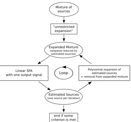
The structure of the algorithm is illustrated in Figure 2. Note that it is a mere extension of SFA in that it does not include new objectives or constraints. We therefore term it xSFA foreXtended SFA.
Additional ICA Steps for Increasing Robustness
Figure 2:Illustration of the xSFA algorithm. The mixture of the input signals is first subjected to a nonlinear expansion that should be chosen sufficiently powerful to allow (a good approximation of) the inversion of the mixture. An estimate of the first source is then obtained by applying linear SFA to the expanded data. The remaining sources are estimated iteratively by removing nonlinear versions of the previously estimated sources from the expanded data and reapplying SFA. If the number of sources is known, the algorithm terminates when estimates of all sources have been extracted. If the number of sources is unknown, other terminal criteria might be more suitable (not investigated here).
If the ∆-values of the sources are very different, the algorithm almost certainly finds the first source. However, because the first source is so much slower than the second, the ∆-values of the productsg(j,1)=g1jg21 of the second source and the
harmonics of the first are similar to the ∆-value of the second source g21 alone, so that the algorithm may not find the second source, but rather a linear mixture ofg21and product solutionsg(j,1). In this case, it is not obvious how the problem
can be tackled, because the signalsg21andg(j,1)are not statistically independent,
so that the usual techniques for linear BSS cannot be expected to disentangle the mixture. In practice, however, second order ICA seems to solve the problem with more than chance level. A possible explanation is that the product solutions – although not statistically independent – should be uncorrelated, probably also when time delays are introduced. Second order ICA relies on the removal of time-delayed correlations, which may in this case help to remove random correlations between the product states and the second source. This situation of possible mixtures of product solutions can also be detected blindly, because after projecting out nonlinear versions of the first source and performing linear SFA, the slowest solution is only likely to be a mixture, if the ∆-value of the second slowest output signal is similar.
Formalization of the xSFA Algorithm
The simulations presented below apply the following scheme to a nonlinear mix-turex(t), t∈ {1, ..., T}of two sourcess(t):
2. Apply linear SFA to the expanded data and store theJ slowest output sig-nalsy(1)j .
3. If the ∆-values of the slowest output signals of SFA are similar, apply second order ICA to the slowest signals to account for possible linear mixtures of similar sources. We chose to perform this step on all signals, whose ∆-value differed from that of the slowest signal by no more than a factor of 1.4.
4. Choose the slowest output signaly(1)1 as a representative ˜s1of the first source.
5. Expand the representative ˜s1 of the first source in monomials of degreeNnl
and whiten the resulting signals. We refer to the resulting nonlinear versions of the first source asnk, k∈ {1, ..., Nnl}.
6. Remove the nonlinear versions of the first source from the SFA output sig-nalsy(1)j
yj(2)(t) =y(1)j (t)−
Nnl
X
k=1
cov(yj(1), nk)nk(t) (35)
and remove principal components with a variance below a given threshold.
7. Apply linear SFA toyj(2)and store the output signalsy(3)j .
8. If the ∆-values of the slowest output signals of the last SFA step are similar, apply second order ICA to the first components ofy(3)j to disentangle possible linear mixtures of the second source with products of the second source and harmonics of the first. We chose to perform this step on all signals, whose ∆-value differed from that of the slowest signal by no more than a factor of 1.7. Choose the output signal with the smallest ∆-value as a representative ˜s2of the second source.
4.2 Simulations
We test the algorithm on two different tasks. The first one is the separation of two audio signals that are subject to a rather complicated mixture. In the second task, we test if the algorithm is able to separate more than two sources.
Sources
We evaluated the performance of the algorithm on two different test sets of audio signals. Data set A consists of excerpts from 14 string quartets by Bela Bartok. Note that these sources are from the same CD and the same composer and con-tain the same instruments. They can thus be expected to have similar statistics. Differences in the ∆-values should mainly be due to short-term nonstationarities. This data set provides evidence that the algorithm is able to distinguish between signals that have similar global statistics based on short-term fluctuations in their statistics.
Data set B consists of 20 excerpts from popular music pieces from various genres, ranging from classical music over rock to electronic music. The statistics of this set is more variable in their ∆-values, in particular they remain different even for long sampling times.
Nonlinear Mixture
Separation of 2 audio signals: We subjected all possible pairs of sources within a data set to a nonlinear invertible mixture that was previously used by Harmeling et al. (2003) and Blaschke et al. (2007):
x1(t) = (s2(t) + 3s1(t) + 6) cos(1.5πs1(t)),
x2(t) = (s2(t) + 3s1(t) + 6) sin(1.5πs1(t)). (36)
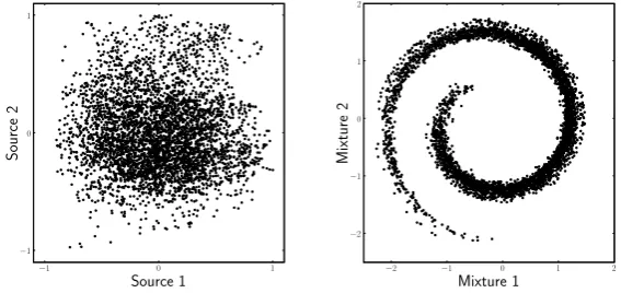
Figure 3 illustrates the spiral-shaped structure of this rather extreme nonlinearity.
Figure 3:The spiral-shaped structure of the nonlinear mixture.Panel A shows a scatter plot of two sources from data set A. Panel B shows a scatter plot of the nonlinear mixture we used to test the algorithm.
This mixture is only invertible if the sources are bounded between -1 and 1, which is the case for the audio data we used. The mixture (36) is not symmetric in s1
and s2. Thus, for every pair of sources, there are two possible mixtures and we have tested both for each source pair.
We have also tested the other nonlinearities that Harmeling et al. (2003) applied to two sources, as well as post-nonlinear mixtures, i.e., linear mixture followed by a point nonlinearity. The performance was similar for all tested mixtures without any tuning of parameters (data not shown). Moreover, the performance remained practically unchanged when we used linear mixtures or no mixture at all. This is in line with the argument that the mixture should be irrelevant to SFA if the function spaceF is sufficiently rich (see section 3).
Separation of more than 2 sources: For the simulations with more than two sources, we used a post-nonlinear mixture by first applying a random rotationOij
to the sources si and then applying a point-nonlinearity to each of the linearly
mixed signals. The nonlinearity we used is arctangent with a scaling parameter:
xj= arctan((
X
Oijsj)/T). (37)
The parameterT determines the degree of the nonlinearity. For these simulations with we normalize the sources to have zero mean and unit variance, to ensure that the degree of nonlinearity is roughly the same for all combinations of sources.
Simulation Parameters
There are several parameters of the algorithm: the degreeNSFAof the expansion used for the first SFA step, the degreeNnlof the expansion for the source removal,
mixtures due to random correlations.
Degree of the expansion in the first SFA step: For the simulations with two sources,we used a polynomial expansion of degreeNSFA= 7, because it has
previ-ously been shown that this function space is sufficient to invert the mixture (36) (Blaschke et al., 2007). For 2-dimensional input signals, this expansion generates a 35-dimensional function space. We kept allJ= 35 output signals of SFA. It is worth noting that the success rate of the algorithm practically unchanged when polynomials of higher order are used. From the theoretical perspective, this is not surprising, because once the function space is sufficiently rich to extract the first harmonics of the sources, the system performs just as good as it could with an unrestricted function space.
For the simulations with more than two sources, we used a polynomial expan-sion of degreeNSFA= 3.
Degree of the expansion for source removal: For the simulations with twoWe sources, we expanded the estimate for the first source in polynomials of degreeNnl=
20, i.e., we projected out 20 nonlinear versions of the first source. Using fewer non-linear versions does not alter the results significantly, as long as the expansion is sufficiently complex to remove those harmonics of the first source that have smaller ∆-values than the second source. Using higher expansion degrees sometimes leads to numerical instabilities, which we accredit to the extremely sparse distribution that result from the application of very high monomials.
For the separation of more than two sources, all polynomials of degreeNnl= 4 of the already estimated sources were projected out.
Variance threshold: After the removal of the nonlinear versions of the first source, there is at least one direction with vanishing variance. To avoid numerical prob-lems caused by singularities in the covariance matrices, directions with variance below = 10−7 were removed. For almost all source pairs, the only dimension that had a variance belowafter the removal was the trivial direction of the first estimated source.
Parameters for second order ICA steps: The algorithm we used for second or-der ICA is TDSEP (Ziehe and M¨uller, 1998). TDSEP relies on the simultaneous diagonalization of multiple time-delayed covariance matrices with different delays. We used time delays that were equally spaced by 100 samples. The maximal delay was 44100 samples, which corresponds to 441 different time delays within 1s. If the training data were shorter than the maximal delay, the total number of delays was limited by the duration of the training data.
The TDSEP step after the first SFA step (step 3 in the scheme above) that should separate linear mixtures of similarly slow sources was only done on those signals whose ∆-value differed by a factor of less than 1.4 from that of the slowest signal. For the TDSEP step that should separate the second source and product solutions (step 7), we used only those signals whose ∆-values differed by a factor of less than 1.7 from the slowest signal. The choice for these two thresholds is conservative. The results do not rely on fine tuning of these parameters.
The simulations were done in PYTHON using the modular data processing toolbox (MDP) developed by Zito et al. (2008).
Performance Measure
neither Gaussian nor stationary (at least not on the time scales we used for train-ing). In this case the algorithm cannot be expected to find the sources themselves, but rather a nonlinearly transformed version of the sources, ideally their lowest harmonics. Thus, the correlation between the output signals of the algorithm and the sources is not necessarily the appropriate measure for the quality of the source separation. Therefore, we also calculated the correlation of the sources with the closest nonlinearly transformed version of its estimate. To this end, we performed a linear regression between each of the sources and a polynomial expansion of the source estimate with highest linear correlation with the source. The corre-lation between this optimally transformed source estimate and the source takes into account possible nonlinear distortions of the source. Almeida (2005) used an equivalent approach, but calculated the signal-to-noise ratio instead of the corre-lation. We considered source reconstruction to be successful, when the associated correlation was above 0.9.
Data Set A Data Set B
Sources
A C
Harmonics
B D
Figure 4:Performance of the algorithm as a function of the duration of the training data. The curves show the percentage of source pairs, for which the algorithm reconstructed 0 (dash-dotted), 1 (dashed), and 2 (solid) of the sources/harmonics. Panels A and B show results for data set A, panels C and D for data set B. Panels A and C show the ability of the algorithm to reconstruct the sources themselves, while B and D show the performance when trying to reconstruct the harmonics of the sources. Statistics cover all possible source pairs that can be simulated (data set A: 14 sources→182 source pairs, data set B: 20 sources→380 source pairs). Note the difference in time scales.
Simulation Results
For data set B, the sources could be reconstructed for 91.7±0.3% (mean±std, n=3 data points for training times 2, 5 and 10s) of the source pairs, but longer training times of at least 2s were necessary. Further research will be necessary to assess the reasons for this. Surprisingly, on average, the sources estimated by the algorithm match the original sources slightly better than the harmonics of the sources. A possible reason might lie in the complexity of the function space. If the relation between the harmonics and the sources is highly nonlinear, the function space may be sufficiently complex to find a good approximation of the sources, but not of the harmonics.
The performance of xSFA is significantly better than that of independent slow feature analysis (ISFA; Blaschke et al., 2007), which also relies on temporal corre-lations and was reported to reconstruct both sources for about 70% of the source pairs. Moreover, it is likely that the performance of xSFA can be further improved, e.g., by using more training data or different function spaces.
The algorithm is relatively fast: On a notebook with 1.7GHz, the simulation of the 182 source pairs for dataset A with 0.2s training sequences takes about 380 seconds, which corresponds to about 2.1s for the unmixing of a single pair.
5 Practical Limitations
There are several reasons why the algorithm can fail, because some of the as-sumptions underlying the theory are not necessarily fulfilled in simulations. In the following, we discuss some of the reasons for failures. The main insights are summarized at the end of the section.
Limited Sampling Time
The theory predicts that some of the output signals reproduce the harmonics of the sources exactly. However, problems can arise if eigenfunctions have (approx-imately) the same eigenvalue. For example, let us assume that the sources have the same temporal statistics, so that the ∆-value of their slowest harmonicsgµ1 is
equal. Then, there is no reason for SFA to prefer one signal over the other. Of course, in practice, two signals are very unlikely to have exactly the same ∆-value. However, the difference may be so small that it cannot be resolved because of limited sampling. To get a feeling for how well two sources can be distinguished, assume there were only two sources that are drawn independently from probability distributions with ∆-values ∆ and ∆+δ. Then linear SFA should ideally reproduce the sources exactly. However, if there is only a finite amount of data, say of total durationT, the ∆-values of the signals can only be estimated with finite precision. Qualitatively, we can distinguish the sources when the standard deviation of the estimated ∆-value is smaller than the differenceδ in the “exact” ∆-values. It is clear that this standard deviation depends on the number of data points roughly as 1/√T. Thus the smallest differenceδmin in the ∆-values that can be resolved has the functional dependence
δmin∼∆α√1
T . (38)
For dimensionality reasons, the exponent α has to take the value α = 3/4, yielding the criterion
δmin
∆ ∼
1
p
T√∆
. (39)
For an interpretation of this equation note that the ∆-value can be interpreted as a (quadratic) measure for the width of the power spectrum of a signal (assuming a roughly unimodal power spectrum centered at zero):
∆(y) = 1
T
Z
˙
y2dt= 1
T
Z
ω2|y(ω)|2dω , (40)
where y(ω) denotes the Fourier transform of y(t). However, the inverse width of the power spectrum is an operative measure for the correlation timeτof the signal, leaving us withτ∼1/√∆. With this in mind, the criterion (39) takes a form that is much easier to interpret:
δmin
∆ ∼
r
τ T =
1
√
Nτ
. (41)
τ characterizes the time scale on which the signal varies, so intuitively, we can cut the signal into Nτ = T /τ “chunks” of duration τ, which are approximately
independent. Equation (41) then states that the smallest relative difference in the ∆-value that can be resolved is inversely proportional to the square root of the numberNτ of independent data “chunks”.
If the difference in the ∆-value of the predicted solutions is smaller thanδmin, SFA is likely not to find the predicted solutions but rather an arbitrary mixture thereof, because the removal of random correlations and not slowness is the es-sential determinant for the solution of the optimization problem. Equation (41) may serve as an estimate of how much training time is needed to distinguish two signals. Note however, that the validity of (41) is questionable for nonstationary sources, because the statistical arguments used above are not valid.
Using these considerations, we can estimate the order of magnitude of training data that is needed for the datasets we used to evaluate the performance of the algorithm. For both datasets, the ∆-values of the sources were on the order of 0.01, which corresponds to an autocorrelation time of approximately 1/√0.01 = 10 samples. Those sources of dataset A that were most similar differed in ∆-value by
δ/∆∼0.05, which requires Nτ = (1/0.05)2 = 400. This corresponds to∼4000
samples that are required to distinguish the sources, which is similar to what was observed in simulations. In dataset B, the problem is not that the sources are too similar, but rather that they are too different in ∆-value, which makes it difficult to distinguish between the products of the second source and harmonics of the first and the second source alone. The ∆-values often differ by a factor of 20 or more, so that the relative difference between the relevant ∆-values is again on the order of 5%. In theory, the same amount of training data should therefore suffice. However, if the sources strongly differ in ∆-value, many harmonics need to be projected out before the second source is accessible, which presumably requires a higher precision in the estimate of the first source. This might be one reason why significantly more training data is needed for dataset B.
Sampling Rate
For discrete data, the temporal derivative is usually replaced by a difference quotient:
˙
y(t)≈y(t+ ∆t)−y(t)
∆t , (42)
where y(t+ ∆t) and y(t) are neighboring sample points and ∆t is given by the inverse of the sampling rater. The ∆-value can then be expressed in terms of the variance of the signal and its autocorrelation function:
∆(y) =hy˙2it≈
2 ∆t2 hy
2i
t− hy(t+ ∆t)y(t)it
= 2r2 hy2it− hy(t+ ∆t)y(t)it
.
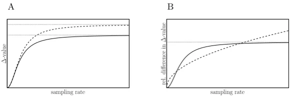
(43) If the sampling is too low, the signal effectively becomes white noise. In this case, the term that arises from the time-delayed correlation vanishes, while the variance remains constant. Thus, for small sampling rates, the ∆-value depends quadratically on the sampling rate, while it saturates to its “real” value if the sampling rate is increased. This behavior is illustrated in Figure 5A. Note that signals with different ∆-values for sufficient sampling rate may have very similar ∆-value when the sampling is decreased too drastically. Intuitively, this is the case if the sampling rate is so low that both signals are (almost) white noise. In this case, there are no temporal correlations that could be exploited, so that SFA returns a random mixture of the signals.
A B
Figure 5:Influence of the sampling rate.(A) Qualitative dependence of the ∆-value of two different signals on the sampling rate. For very low sampling rates, both sig-nals become white noise and the ∆-value quadratically approaches zero. Sigsig-nals that have different ∆-values for sufficiently high sampling rates may therefore not be distinguishable if the sampling rate is too low. The dotted lines indicate the “real” ∆-values of the signals. Note: It may sound counterintuitive that the ∆-value drops to zero with decreasing sampling rate, as white noise should be regarded as a quickly varying signal. This arises from taking the sampling rate into account in the temporal derivative (43). If the derivative is simply replaced by the difference between adjacent data points, the ∆-value approaches 2 as the sampling rate goes to zero and decreases with the inverse square of the sampling rate as the sampling rate becomes large. (B) Sampling rate dependence of the “resolution” of the algorithm for a fixed number of training samples. The solid line shows the qualitative dependence of the relative difference in ∆-value of two signals as a function of the sampling rate and the dashed line shows the qualitative behavior of the minimal relative difference in ∆-value that can be resolved. The signals can only be separated by SFA if the resolvable difference (dashed) is below the expected relative difference (solid). Therefore an inter-mediate sampling is more efficient. The dotted line indicates the “real” ratio of the ∆-values.
in ∆-value that can be resolved is proportional to 1/√T ∼√r. But why do low sampling rates lead to a better resolution? The reason is that for high sampling rates, neighboring data points have essentially the same value. Thus, they do not help in estimating the ∆-value, because they do not carry new information.
In summary, the sampling rate should ideally be in an intermediate regime. If the sampling rate is too low, the signals become white noise and cannot be distin-guished, while too high sampling rates lead to high computational costs without delivering additional information. This is illustrated in Figure 5B.
Density of Eigenvalues
The problem of getting random mixtures instead of the optimal solutions is of course most relevant in the case where the sources, or more precisely, the slow-est non-constant harmonics of the sources have similar ∆-values. However, even when the sources are sufficiently different, this problem eventually arises for the higher-order solutions. To quantify the expected differences in ∆-value between the solutions, we define adensityρ(∆) of the ∆-values as the number of eigenvalues expected in an interval [∆,∆ +δ], divided by the interval lengthδ. A convenient way to determine this density is to calculate the number R(∆) of solutions with eigenvalues smaller than ∆ and then take the derivative with respect to ∆.
In the Gaussian approximation, the ∆-values of the harmonics are equidistantly spaced, cf. (31). As the ∆-value ∆iof the full product solutiongiis the sum of the ∆-values of the harmonics, the condition ∆i<∆ restricts the indexito lie below a hyperplane with the normal vectorn= (λ11, ..., λS1)∈RS:
X
µ
iµλµ1=i·n<∆. (44)
Because the indices are homogeneously distributed in index space with density one, the expected number of solutions with ∆<∆0 is simply the volume of the
subregion in index space for which equation (44) is fulfilled:
R(∆) = 1
S!
S
Y
µ=1
∆
λµ1
. (45)
The density of the eigenvalues is then given by
ρ(∆) = ∂R(∆)
∂∆ = 1 (S−1)!
" Y
µ
1
λµ1
#
∆S−1. (46)
As the density of the eigenvalues can be interpreted as the inverse of the expected distance between the ∆-values, the distance and thus the separability of the so-lutions with a given amount of data declines as 1/∆S−1. In simulations, we can
expect to find the theoretically predicted solutions only for the slowest functions, higher order solutions tend to be linear mixtures of the theoretically predicted functions. This is particularly relevant if there are many sources, i.e., ifS is large. If the sources are not Gaussian, the dependence of the density on the ∆-value may have a different dependence on ∆ (e.g., for uniformly distributed sources
ρ(∆)∼∆S/2−1). The problem of decreasing separability, however, remains.
Function Space
Because the nature of the nonlinear mixture is not knowna priori, it is diffi-cult to choose an appropriate function space. We used polynomials with relatively high degree. A problem with this choice is that high polynomials generate ex-tremely sparse data distributions. Depending on the input data at hand, it may be more robust to use other basis functions such as radial basis functions or kernel approaches, although for SFA, these tend to be computationally more expensive.
The suitability of the function space is one of the key determinants for the quality of the estimation of the first source. If this estimate is not accurate but has significant contributions from other sources, the nonlinear versions of the estimate that are projected out are not accurate, either. The projection step may thus remove aspects of the second source and thereby impair the estimate of the second source. We expect that for many sources, these errors will accumulate so that estimates for faster sources will not be trustworthy. This problem might be further engraved by the increasing eigenvalue density discussed above.
Summary
In summary, we have discussed four factors that have an influence on simulation results:
Limited sampling time: If the algorithm can distinguish two sources with similar ∆-values depends on the amount of data that is available. More precisely, to separate two sources with ∆-values ∆ and ∆ +δ, the duration T of the training data should be on the order ofT ∼τ(∆/δ)2 or more. Here,τ is the autocorrelation time of the signals, which can be estimated from the ∆-value of the sources:τ ≈1/√∆.
Sampling rate Because the algorithm is based on temporal correlations, the sam-pling rate should of course be sufficiently high to have significant correlations between subsequent data points. If the numberTof samples that can be used is limited by the memory capacity of the computer, very high sampling rates can be a disadvantage, because the correlation timeτ (measured in samples) of the data is long. Consequently, the numberT /τ of “independent data chunks” is smaller than with lower sampling rates, which may impair the ability of the algorithm to separate sources with separate similar ∆-values (see previous point).
Density of eigenvalues: The problem of similar ∆-values is not only relevant when the sources are similar, because the algorithm also needs to distinguish the faster sources from products of these sources with higher-order harmonics of the lower sources. To estimate how difficult this is, we have argued that, for the case of Gaussian sources, the expected difference between the ∆-values of the output of SFA declines as 1/∆S−1, whereS is the number of sources.
Separating a source from the product solutions of lower-order sources there-fore becomes more difficult with increasing the number of sources.
6 Discussion
In this article, we have extended previous theoretical results on SFA to the case where the input data are generated from a set of statistically independent sources. The theory shows that (a) the optimal output of SFA consists of products of signals, each of which depends on a single source only and that (b) some of these harmonics should be monotonic functions of the sources themselves. Based on these predictions, we have introduced the xSFA algorithm to iteratively reconstruct the sources, in theory from arbitrary invertible mixtures. Simulations for a rather complicated nonlinear mixture of two audio sources have shown that the algorithm extracts both sources for 90% percent of the source pairs. The performance is substantially higher than the performance of independent slow feature analysis (ISFA; Blaschke et al., 2007), another algorithm for nonlinear BSS that relies on temporal correlations.
xSFA is relatively robust to changes of the implementation details. Neither a higher degree of the expansion before the first SFA step nor the removal of more nonlinear versions of the first source change the reconstruction performance sig-nificantly. It should be noted, however, that polynomial expansions - as used here - become problematic if the degree of the expansion is too high. The resulting expanded data contain directions with very sparse distributions, which can lead (a) to singularities in the covariance matrix (e.g., for Gaussian signals with limited sampling,x20andx22 are almost perfectly correlated) and (b) to sampling prob-lems for the estimation of the required covariances because the data are dominated by few data points with high values. Note, that this problem is not specific to the algorithm itself, but rather to the expansion type used. Other expansions such as radial basis functions may be more robust. The relative insensitivity of xSFA to parameters is a major advantage over ISFA, whose performance depended crucially on the right choice of a trade-off parameter between slowness and independence.
Many algorithms for nonlinear blind sources separation are designed for specific types of mixtures, e.g., for post-nonlinear mixtures (for an overview of methods for post-nonlinear mixtures see Jutten and Karhunen, 2003). In contrast, our algo-rithm should work for arbitrary instantaneous mixtures. As previously mentioned, we have performed simulations for a set of instantaneous nonlinear mixtures and the performance was similar for all mixtures. The only requirements are that the sources are distinguishable based on their ∆-value and that the function space accessible to SFA is sufficiently complex to invert the mixture. Note that the algorithm is restricted to instantaneous mixtures. It cannot invert convolutive mixtures because SFA processes its input instantaneously and is thus not suitable for a deconvolution task.
We have presented simulations for two sources only. In theory, the algorithm should be able to separate mixtures of more sources as well. In practice, however, the number of reconstructable sources may be limited because of accumulating errors as discussed in section 5. Further simulations are needed to assess the performance of the algorithm for more sources.
It would be interesting to see if the theory for SFA can be extended to other algorithms. For example, given the close relation of SFA to TDSEP (Ziehe and M¨uller, 1998), a variant of the theory may apply to the kernel version of TDSEP (Harmeling et al., 2003).
References
L.B. Almeida. Separating a Real-Life Nonlinear Image Mixture.The Journal of Machine Learning Research, 6:1199–1229, 2005.
A.J. Bell and T.J. Sejnowski. An information maximization approach to blind separation and blind deconvolution. Neural Computation, 7:1129–1159, 1995.
A. Belouchrani, K. Abed-Meraim, J.-F. Cardoso, and E. Moulines. A blind source separa-tion technique using second order statistics. IEEE Transactions on Signal Processing, 45:434–444, 1997.
P. Berkes and L. Wiskott. Slow feature analysis yields a rich repertoire of complex cells.
Journal of Vision, 5(6):579–602, 2005.
T. Blaschke and L. Wiskott. CuBICA: Independent component analysis by simultane-ous third- and fourth-order cumulant diagonalization. IEEE Transactions on Signal Processing, 52(5):1250–1256, May 2004.
T. Blaschke, P. Berkes, and L. Wiskott. What is the relation between slow feature analysis and independent component analysis? Neural Computation, 18(10):2495–2508, 2006.
T. Blaschke, T. Zito, and L. Wiskott. Independent slow feature analysis and nonlinear blind source separation. Neural Computation, 19(4):994–1021, 2007.
S. Choi. Differential learning algorithms for decorrelation and independent component analysis.Neural Netw, 19(10):1558–1567, Dec 2006. doi: 10.1016/j.neunet.2006.06.002.
R. Courant and D. Hilbert. Methods of mathematical physics Part I. Wiley, 1989.
M. Franzius, H. Sprekeler, and L. Wiskott. Slowness and sparseness lead to place, head-direction, and spatial-view cells. PLoS Computational Biology, 3(8):e166, Aug 2007.
S. Harmeling, A. Ziehe, M. Kawanabe, and K.-R. M¨uller. Kernel-based nonlinear blind source separation.Neural Computation, 15:1089–1124, 2003.
A. Hyv¨arinen. Fast and robust fixed-point algorithms for independent component analysis.
IEEE Transactions on Neural Networks, 10:626–634, 1999.
A. Hyv¨arinen and P. Pajunen. Nonlinear independent component analysis: Existence and uniqueness results.Neural Networks, 12(3):429–439, 1999.
A. Hyv¨arinen, J. Karhunen, and E. Oja.Independent Component Analysis. Wiley, 2001.
C. Jutten and J. Karhunen. Advances in nonlinear blind source separation. Proc. of the 4th Int. Symp. on Independent Component Analysis and Blind Signal Separation (ICA2003), pages 245–256, 2003.
L. Molgedey and H. G. Schuster. Separation of a mixture of independent signals using time delayed correlations. Physical Review Letters, 72(23):3634–3637, 1994.
L. Wiskott. Learning invariance manifolds. In L. Niklasson, M. Bod´en, and T. Ziemke, editors, Proceedings of the 8th International Conference on Artificial Neural Net-works, ICANN’98, Sk¨ovde, Perspectives in Neural Computing, pages 555–560, London, September 1998. Springer.
L. Wiskott and T.J. Sejnowski. Slow feature analysis: unsupervised learning of invariances.
Neural Computation, 14:715–770, 2002.
L. Wiskott. Slow feature analysis: A theoretical analysis of optimal free responses.Neural Computation, 15(9):2147–2177, September 2003.
A. Ziehe and K.R. M¨uller. TDSEP–an efficient algorithm for blind separation using time structure.Proc. Int. Conf. on Artificial Neural Networks (ICANN ’98), pages 675–680, 1998.