c
EDP Sciences, 2009
DOI: 10.1140/epjconf/e2009-00923-x
T
HE
E
UROPEAN
P
HYSICAL
J
OURNAL
CONFERENCES
Solar magnetic activity: Topologically explored
H. Lundstedt
Swedish Institute of Space Physics, Lund, Sweden
Abstract. Solar magnetic activity is the driver of solar and space weather and with its effects. It is therefore of great importance to be able to predict it. How-ever, before being able to make predictions, we need to know the present state. Topological methods are presented that could give a more precise and complete description of the present; the over all, and the magnetic dynamo activity state of the Sun.
1 Introduction
Solar magnetic activity is the driver of the space weather and its effects [13, 14]. It is therefore of great importance to be able to predict it [15, 17].
However, before we can make predictions we need to know the present state. We also have to define what we mean by solar magnetic activity and the state [18].
A magnetic field is represented by a continuous vector function,B(r). The lines of force are defined, in terms ofB(r), as the two-parameter family of solutions of the two equations,
dx Bx =
dy By =
dz
Bz. (1)
In a fluid with infinite electrical conductivity, the topology of the lines is invariant, the lines of force being carried with the fluid. In the presence of resitivity the topology is not invariant. The magnetic field transmits stresses between regions of material particles and fluids. It is these stresses (described by the Maxwell stress tensor)
Mi,j∼=−δijB2/8π+BiBj/4π (2)
that are responsible for the non-equilibrium and the continual activity of fluids in astrophysical bodies [21].
The topological properties of the lines of force of a magnetic field Bi(r) determine the activity of that field. Only the most symmetrical field topologies possess equilibrium. The field is being compelled to a life of dynamical dissipation. Magnetic fields in nature are generally stochastic, lacking the symmetric topologies necessary for equilibrium. The topological non-equilibrium is the cause of the solar magnetic activity. Solar magnetic activity has therefore been explored with the use of topological methods by many [12]. Let me first describe some basics of topology before start applying it.
2 Topology
Topology is the mathematical study of the ’properties’ that are preserved through deforma-tions, twisting and stretching of objects. Tearing is not allowed. Topology is the study of ’spatial objects’, such as curves, knots (= non-self-intersecting curves that are embedded in
Article published by EDP Sciences and available at http://www.epj-conferences.org
three dimensions), surfaces, manifolds (= topological spaces that are locally Euclidean i.e., around every point, there is a neighborhood that is topologically the same as the open unit ball in Rn), and phase spaces (= for a system of nfirst-order ordinary differential equations, the 2n-dimensional space consisting of the possible values of (x1,x1, x2,˙ x2, . . . , x˙ n,x˙n) is known as its phase space). Topology can be used to abstract the ‘inherent connectivity’ of objects while ignoring their detailed form. Topology is formally defined in terms of set operations. Let X
be a set. A topology on X is a collection T of subsets of X, called the open sets. The set X
together with a topology T is called a topological space. An open set is a set for which every point in the set has a neighborhood lying in the set. A subsetA is dense in a spaceX if and only ifA intersects every nonempty open set inX.
Topology is today divided into many subdivisions such as, point-set, algebraic, differential topology and knot theory.
Point set topology studies points and sets in topological spaces, and continuous functions between topological spaces.
In algebraic topology, one uses algebra as a tool to study topology. Given a topological space, one can determine the number of pieces (or components) of the space. The number of components is called a ‘topological invariant’, because any two topological equivalent spaces have the same number of components. A topological invariant is a property that depends only on the topology of the topological space and nothing else. The ‘fundamental group’ is a topological invariant that can be regarded as the space of all essentially different loops in a topological space.
The over all complexity of the magnetic flux distribution may be described by the topological connectivity between magnetic flux regions [12, 19].
We will focus of differential topology, knot theory and dynamical systems.
2.1 Differential topology – Poincar´e Index
In differential topology the interactions between topology and calculus are studied, including analysis of differential equations. If V is a vector field with zero curl on an open subset U of
R2, then the integral of V around a loop provides topological information about the open set U and the loop. If the integral e.g. is not zero, then the space U must have a “hole” and the loop must go around the hole.
We say that two maps are homotopic () if one can be continuously deformed to the other. The concept of homotopy is then used to develop the winding number (W(γ, P)), i.e. of a loop
γ:I→R−{P}around a pointP, which is simply the number of times the loopγ(of radiusr) winds around the pointP. Ifγ0γ1⇔W(γ0, P) =W(γ1, P). The index ofV atP is defined asIndexP(V) =W(V ◦γr,0), where 0 denotes the origin inR2.
Poincar´e-Index Theorem says: Suppose thatU is an open set inR2, thatD is a closed disk inU, and thatV is a vector field onU having only isolated zeros, all of which are contained in
D. Letγdenote the pathγ(s) = (x0, y0) + (rcos(2πs), rsin(2π)), where (x0, y0) is the center of
Dandris the radius ofD. Then the winding numberW(V◦γ,0) =P∈ZIndexP(V), where
P is an isolated zero of the vector field.
Path integrals of vector fields (magnetic fields) can then be interpreted as the winding number. The Poincar´e index gives information about the space around the null points.
2.2 Differential manifolds – Poincar´e Hopf Theorem
IfU is an open subset ofRn, then a vector field onU is a functionV :U →Rn that assigns to each pointx∈U a vectorV(x).
A smooth surface is a surface in Rn that has a tangent plane at each point. The tangent plane to S at a point p is denotedTpS.
A vector field V on a surface S is a continuous map V : S → T S that takes each point
p∈S to a vectorV(p)∈TpM.
A map is said to be a diffeomorphism if it is a homeomorphism (i.e. preserves the topological properties) and additionally, the map and its inverse are continuously differentiable. Suppose thatX andY are open subsets ofR2and thatf :X →Y is a diffeomorphism. For vector field
V onX, define the push forward ofV byf to be the vector fieldf∗V = (df)V. If (u, v) =f(x, y)
then
f∗V(x, y) = (df(x,y))V(x, y). (3) df(x,y)may be calculated from the Jacobian matrix Jf(x, y).
Poincar´e - Hopf Theorem: If a vector field on a surface S has only isolated zeros then the sum of the indices of the zeros is equal to χ(S), where χ(S) is the Euler characteristic (χ(Circle) = 0, χ(Disk) = 1,χ(Sphere) = 2 andχ(T orus) = 0).
2.3 Knot theory – Linking number
The Gauss Linking number is given by,
L(C1, C2) = 1 4π
C1
C2
(¯xC1−x¯C2)·(dx¯C1×dx¯C2)
|¯xC1−x¯C2|3
(4)
where the two loopsC1andC2are described by two three-vectors ¯xC1and ¯xC2. L is not changed,
being an invariant, as the two loops are deformed as long as they do not intersect each other. The Linking number was already derived by Gauss, using electromagnetic theory [20]. The integral ofB along the curveC1andC2 gives,
C1
¯
B·dl¯ =−Iµ0 4π
C1
C2
(¯r1−r2¯ )×dl2¯ ·dl1¯
|r1¯ −¯r2|3 · (5)
However, Ampere’s law gives,
C1
¯
B·dl¯ =
S ¯
∇ ×B¯·ds¯=µ0
S
¯j·s¯=µ0mI (6)
where m is the algebraic sum of times the wire cuts the surface S, and also Linking number. A much simpler method for computing the linking number of two loops (curves) is to make use of the fact that knots can be represented by plane diagrams. These projections of the knots onto a plane that preserves crossing information. The linking number is then half the sum of the signed crossings.
L(C1, C2) =1 2
i
σi(C1, C2) (7)
whereσi(C1, C2) =σi(C2, C1) =±1 is assigned to each crossings. The helicity of a magnetic field can be expressed as
H=
V A·BdV (8)
whereAis the vector potential andB=∇ ×A.
Using a geometric invariant of a space curve (writhing number) [2] decomposed the helicity of a magnetic field into the sum of “twist” and “kink” helicities and defined the helicity of open field structures. A theorem of knot theory was used that states that the linking number of two curvesX andY (LXY) without common points can be written as the sum of the twist number
TW and the writhing numberWR.
2.4 Dynamical systems
The basic goal of the theory of dynamical systems is to understand the eventual or asymptotic behavior of an interative process. If the process is a differential equation whose independent variable is time, then the theory attempts to predict the ultimate behavior of solutions of the equation in either the distant future (t→+∞) or distant past (t→ −∞).
A pair{ft, M}, t∈RorR+ in the case of continuous time, andt∈ZorZ+in the case of discrete time is called a dynamical system inM is a complete metric space and for eacht, ftis a continuous map fromM intoM satisfying the (semi)-group property i.e.ft1+t2 =ft1◦ft2 = ft2◦ft1 [1, 11].
A dynamical system is said to be chaotic (Devaney chaotic) [6] if there exists at least one dense orbit and a set of periodic orbits is dense. Topological invariants of periodic orbits, such as the Linking number, can be used to identify the strange attractor and the stretching and squeezing mechanisms [8].
3 The solar state – topologically explored
We will now continue by applying these topological methods to describe the magnetic state of a solar active region, the whole Sun and the solar dynamo cycle.
3.1 The state of an active region
An active region’s capability to produce solar flares and coronal mass ejections is related to the complexity of the magnetic field, the magnetic gradient (energy build-up), the site relative to the neutral line and existence of emerging flux regions (triggers). The energy, released in the events, is stored in the twisted magnetic field.
3.1.1 Transequatorial loops and helicity
Twists and helicity of coronal mass ejection flux loops have been described by topological knots [2, 22, 24].
In [4] they calculated the helicity patterns of 43 pairs of active regions that were connected by transequatorial loops. The helicity patterns were quantified by the parameters, force-free field coefficientαand the current helicity component hc. A correlation of 85% between these parameters was found. These parameters will be used for state description.
3.1.2 Activity and null points on manifolds
Nullpoints have been associated with the occurrence of solar flares and coronal mass ejections (CMEs). The Poincar´e index characterizes the space around nullpoints and has been used for studies of solar flares and CMEs [5, 23, 27, 28].
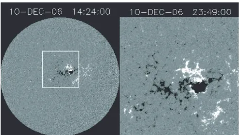
A study of vector fields, null points on manifolds for an active region, is in progress. We selected the active region 10930 (Fig. 1), an active region with a simple bipolar magnetic structure, which however produced intense X-ray flare activity in December 2006.
3.2 The state of the whole Sun’s magnetic activity
Fig. 1.Active region 10930 in December 2006. Courtesy ESA/NASA MDI/SOHO.
Fig. 2. Synoptic map of subsurface flow, surface magnetic field contours and coronal flare activity during the Halloween events of October 2003.
In [10], we showed in synoptic maps how occurrence of flares is related to strong down-flows using helioseismic observations (Fig. 2).
In [15] we outlined how a new indicator can be constructed showing not just the surface solar activity, but the whole Sun’s activity. Helioseismic observations show how activity starts below the solar surface, appearing on surface and is connected to what happens in the corona. Multi-Resolution Analysis (MRA) of synoptic maps below solar surface, on the surface, and in the corona can then be used to extract activity features [17]. All these 3D features can then be related to each other with the use of knowledge-based neural networks [17].
The whole Sun’s magnetic state depends also on the long-term dynamo state. Let us there-fore examine that in next section.
3.3 The state of the solar cycle
Synoptic maps and longitudinally averaged maps of the solar magnetic fields are a very powerful way of visualizing the solar cycle activity.
In [17] we described a multiresolution analysis of averaged synoptic maps for the period 1976 up to present, observed at Wilcox Solar Observatory (WSO), Stanford University. MRA of magnetic fields at sunspot area latitudes, sub-polar latitudes, and at polar latitudes, show how activity varies for different latitudes and scales. We observe how magnetic flux is transported from active regions at sunspot latitudes to polar regions. The longitudinally averaged synoptic maps (Fig. 3) showing the transport of the magnetic flux, is also a picture of the variation of the solar magnetic activity. It can be used for predictions of the next sunspot cycle.
Fig. 3.Longitudinally Averaged Magnetic field (G) observed at Wilcox Solar Observatory.
( ) (+ )
(+ )
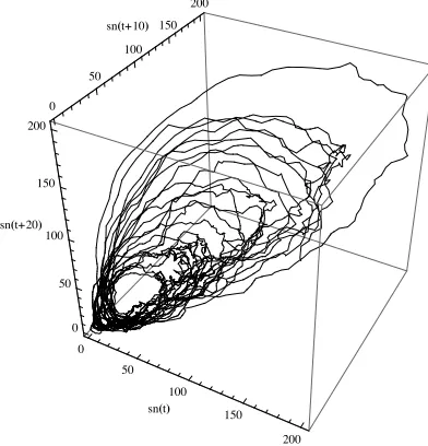
Fig. 4.The dynamic system represented by the monthly sunspot numbers 1749–2008.
weak, as weak as around 1900. This estimate is in accordance to what we found in wavelet ampligram studies [15]. However, even predictions of a strong cycle exists [7].
The NOAA/NASA/ISES Cycle 24 Prediction Panel presented the first prediction on April 25th, 2007. Half of the panel predicts a moderately strong cycle of 140 sunspots plus or minus 20, expected to peak in October of 2011. The other half predicts a moderately weak cycle of 90 sunspots, plus or minus 10, peaking in August of 2012. Both groups predict a minimum in March 2008 plus minus six months.
The difficulties in predicting cycle 24 clearly show the lack of theoretical understanding and data. In this article we also want to stress the lack of precise and complete description of the state. We believe that can be improved by using Topology.
3.3.1 Solar cycles and dynamical systems
( ) ( + )
( + )
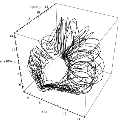
Fig. 5.The dynamic system represented by the14C, 1500–1950, i.e., including the Maunder minimum (1645–1715).
( ) ( + )
( + )
Fig. 6. The dynamical system represented by the output of a MHD model (mean squared toroidal field).
The sunspot data cover the period 1749 up to present. The so called Maunder minimum is therefore not included.
We therefore used 14C to illustrate the Maunder minimum. The data cover the period 1500–1950 [16]. Figure 5 shows a time delay plot, and the embedding.
In [3] they explain the modulation of the solar cycle owing to either stochastic or determin-istic processes. An mean-field αω-dynamo model operating primarily in the region around the base of the solar convection zone. This dynamo model includes the feedback, via the azimuthal component of the Lorenz force, of the mean magnetic field upon the differential rotation. This nonlinear feedback is sole driver of the modulation in the magnetic activity cycle.
2
1
0
1
2
x 2
1 0
1 2
y 1.0
0.5 0.0 0.5
z
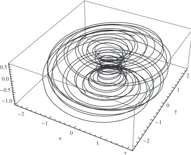
Fig. 7. The dynamical system represented by a low order Lorenz model output for a quasiperiodic state (λ= 0.4, µ= 1.7, a= 3, c=−0.4, d= 2.4, ω= 20.25, µ=Ω1/2).
–2 –1 0 1 2
–0.5 0.0 0.5
x
z
Poincaré section
Fig. 8.The Poincar´e section of the Lorenz low order model output. Omega = 2.89.
∂B
∂t =∇ ×(αB+U×B−β∇ ×B). (10)
The evolution equation for the velocity perturbationV showing the Lorenz force is given by,
∂V ∂t =
1
µ0ρ[(∇ ×B)×B]·eφ+. . . (11)
The mean squared toroidal field output of that MHD model is used for the time-delay plot of Figure 6. Here we see an attractor.
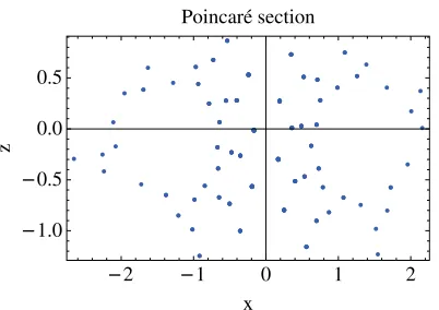
In [26] they describe the modulation of the solar cycle and the occurrence by using a low order dynamic system of Lorenz equation type. The toroidal (BT) and poloidal fields (BP) are represented by the x and the y coordinates respectively. The hydrodynamical information is given by thezcoordinate.
˙
z=µ−z2−(x2+y2) +cz3 (12)
˙
x=λx−ωy+azx+dz(x2+y2) (13) ˙
y=λy+ωx+azy. (14)
–2 –1 0 1 2
–1.0
–0.5 0.0 0.5
x
z
Poincaré section
Fig. 9. The Poincar´e section of the Lorenz low order model output approaching a chaotic state. Omega = 4.0.
We solved the Lorenz equation for values corresponding to a quasiperiodic state (Fig. 7). Poincar´e sections (Fig. 8 and Fig. 9) may then show the development toward a chaotic state.
When the activity, the dynamic system, enters a chaotic state the strange attractor may also be described by the Linking number.
4 Summary
We have suggested to describe the state of active regions by calculating the helicity patterns and null points. We have also suggested to describe the state of the solar cycle by dynamical systems, and several examples were given.
These descriptions will then be presented to a trained knowledge-based neural network predicting the solar state [17, 18].
When vector magnetic field data from Solar Dynamics Observatory [9] will be available, that data will be used.
We are grateful to the following providers of data; ESA/NASA SOHO/MDI team, Wilcox Solar Observatory, Stanford, RWC Belgium, Hoyt Schatten for Rg, NOAA, SWPC and Steve Tobias, UK.
References
1. V. Afraimovich, S.-B. Hsu, Lectures on Chaotic Dynamical Systems, Studies in Advanced Mathematics, AMS, IP, Vol. 28 (2003)
2. M.A. Berger, C. Prior, J. Phys. A: Math. Gen.39, 8321 (2006) 3. P.J. Bushby, S. Tobias, ApJ (2007) (accepted)
4. J. Chen, S. Bao, H. Zhang, Solar Phys. (2007)doi:10.1007/s11207-007-007-0284-9 5. Y. Cui, R. Li, L. Zhang, Y. He, H. Wang, Solar Phys.237, 45 (2006)
6. R.L. Devaney,An Introduction to Chaotic Dynamical Sstems, 2nd edn. (Westview Press, Advanced Book Program, 2003)
7. M. Dikpati, G. de Toma, P.A. Gilman, Geophys. Res. Lett.33, L05102 (2006)
8. R. Gilmore, M. Lefranc, The Topology of Chaos – Alice in Strech and Squeezeland (Wiley-Interscience Publ., 2002)
9. J.T. Hoeksema, and the HMI Magnetic Team, The HMI Magnetic Field Measurement Program, presentation at SDO Team Meeting, March 25–28, Napa, California (2008)
11. A. Katok, B. Hasselblatt, Introduction to the Modern Theory of Dynamical Systems, edited by G.-C. Rota, Vol. 54 (Cambridge Univ., Press, 2006)
12. D.W. Longcope, Living Rev. Solar Phys.2, 7 (2005) 13. H. Lundstedt, Adv. Space Res.36, 2516 (2005)
14. H. Lundstedt, Adv. Space Res.37, 1182 (2006a)doi:10.1016/j.asr.2005.10.023 15. H. Lundstedt, Adv. Space Res.38, 862 (2006b)
16. H. Lundstedt, L. Liszka, R. Lundin, R. Muschler, Ann. Geophys.24, 1 (2006c) 17. H. Lundstedt,On the prediction of solar magnetic activity, OPOCE (2007) 18. H. Lundstedt, Acta Geophys. (2008)
19. R.C. Maclean, Topological Structure of the Magnetic Solar Corona, thesis, Univ. of St. Andrews, 15th September (2006)
20. C. Nash,Topology in physics in a historical essay in History of Topology, edited by I.M. James (Oxford University, UK, Elsevier, 1999)
21. E. Parker,Cosmical Magnetic Fields, Their Origin and their Activity (Oxford University Press, 1979)
22. S. Regnier, T. Amari, R.C. Canfield, A&A442, 345 (2005) 23. S. Regnier, C.E. Parnell, A.L. Haynes, A&A484, L47 (2008)
24. D. Rust, Helicity Conservation, in AGU Geophys. Monograph 99, Coronal Mass Ejections (1997), p. 119
25. L. Svalgaard, E.W. Cliver, Y. Kamide, Geophys. Res. Lett.32(2005) 26. S. Tobias, N.O. Weiss, V. Kirk, Mon. Not. R. Astron. Soc.273, 1150 (1995) 27. H. Wang, J. Wang, A&A3131, 285 (1996)