Nat. Hazards Earth Syst. Sci., 14, 2321–2335, 2014 www.nat-hazards-earth-syst-sci.net/14/2321/2014/ doi:10.5194/nhess-14-2321-2014
© Author(s) 2014. CC Attribution 3.0 License.
Stochastic daily precipitation model with a heavy-tailed component
N. M. Neykov1, P. N. Neytchev1, and W. Zucchini2
1National Institute of Meteorology and Hydrology, Bulgarian Academy of Sciences,
Tsarigradsko Shose 66, Sofia 1784, Bulgaria
2Department of Economic Sciences, Georg-August-Universität, Göttingen, Germany
Correspondence to: N. M. Neykov ([email protected])
Received: 31 October 2013 – Published in Nat. Hazards Earth Syst. Sci. Discuss.: 10 February 2014 Revised: 26 June 2014 – Accepted: 23 July 2014 – Published: 3 September 2014
Abstract. Stochastic daily precipitation models are
com-monly used to generate scenarios of climate variability or change on a daily timescale. The standard models consist of two components describing the occurrence and intensity series, respectively. Binary logistic regression is used to fit the occurrence data, and the intensity series is modeled us-ing a continuous-valued right-skewed distribution, such as gamma, Weibull or lognormal. The precipitation series is then modeled using the joint density, and standard software for generalized linear models can be used to perform the computations. A drawback of these precipitation models is that they do not produce a sufficiently heavy upper tail for the distribution of daily precipitation amounts; they tend to underestimate the frequency of large storms. In this study, we adapted the approach of Furrer and Katz (2008) based on hybrid distributions in order to correct for this short-coming. In particular, we applied hybrid gamma–generalized Pareto (GP) and hybrid Weibull–GP distributions to develop a stochastic precipitation model for daily rainfall at Ihtiman in western Bulgaria. We report the results of simulations de-signed to compare the models based on the hybrid distribu-tions and those based on the standard distribudistribu-tions. Some po-tential difficulties are outlined.
1 Introduction
Stochastic precipitation models are important for forecasting and simulation purposes in climate, hydrological and envi-ronmental system studies in modeling runoff, soil water con-tent, crop growth, droughts and floods. These models can aid in understanding the performance of these systems un-der specific precipitation regimes. Depending on the required
precipitation timescale, various models, such as hourly, daily, weekly, monthly, seasonal or annual, have been developed to quantify complex precipitation features; see Srikanthan and McMahon (2002) and Yang et al. (2005). Once the model has been calibrated at a given site, one uses it to generate long sequences of artificial precipitation at that site. These sequences can be used to estimate statistics relating to pre-cipitation events in exactly the way one would do if a long sequence of real precipitation data were available. As a con-sequence, better risk management strategies and decision-making capabilities can be developed.
In the following, we shall consider precipitation models on daily timescales only. From a statistical point of view, daily precipitation totals are time series with mixed densities, comprising a discrete component at zero (for dry days) and a continuous positive real-valued component (for rain days). A standard technique of analyzing the series is to decompose it into two components, namely the occurrence and the inten-sity processes (Stern and Coe, 1984), and then to model these separately using standard generalized linear model (GLMs) techniques. The occurrence series, consisting of dry and wet states, is modeled by an autoregressive binary logistic regres-sion, and the intensity series by a continuous-valued right-skewed distribution such as gamma, Weibull, lognormal or a mixture of exponential distributions. More precisely, model-ing the occurrence series means modelmodel-ing the transition prob-abilities of the two-state first- or higher-order Markov chain (Gabriel and Neumann, 1962; Katz, 1977). The daily pre-cipitation amounts are then modeled using the joint density of the two components. The seasonal behavior of precipita-tion is accommodated by allowing the model parameters to vary over the year using a finite Fourier representation (Coe and Stern, 1982; Stern and Coe, 1984; Woolhiser, 1992). The
parameters can also be modeled as functions of covariates, e.g., atmospheric factors such as the North Atlantic Oscil-lation, the El Nino–Southern OscilOscil-lation, pressure, humid-ity, temperature, and wind speed, or as slowly varying trend functions over the years. The occurrence (the state transition probabilities) and intensity model components therefore be-come non-stationary. The required computations can be car-ried out using standard software procedures for GLMs and generalized additive models (GAMs), e.g., McCullagh and Nelder (1989), Hastie and Tibshirani (1990) and Fahrmeir and Tutz (2001). The properties and applicabilities of such models on different timescales are discussed by Brandsma and Buishand (1997), Katz and Parlange (1998), Grunwald and Jones (2000), Hyndman and Grunwald (2000), Beckman and Buishand (2002), Chandler and Wheater (2002), Chan-dler (2005), Yang et al. (2005) and Furrer and Katz (2007), to name a few. Reviews of stochastic precipitation modeling can be found in Woolhiser (1992), Wilks and Wilby (1999), Srikanthan and McMahon (2002) and Maraun et al. (2010).
It is well known that the above continuous distributions tend to underestimate the heavy precipitation. Furrer and Katz (2008) developed a flexible approach, based on gamma and GP distributions, in order to model the whole spectrum of precipitation intensities. A gamma distribution (with co-variates) is fitted to the entire intensity data, and then a GP distribution (again with covariates) is fitted to the observa-tions above an appropriately chosen threshold,u. The two es-timated density functions are spliced continuously atuby us-ing the gamma density below the threshold and the GP den-sity (with an estimated shape parameter and a modified scale parameter estimate) above the threshold. The approach of Furrer and Katz (2008) is general, and so other right-skewed distributions, such as Weibull or inverse Gaussian, can be used instead of the gamma one. These authors pointed out some of the difficulties with the procedure, e.g., that thresh-old selection for splicing the distributions is purely subjec-tive. Carreau and Bengio (2009) proposed another hybrid dis-tribution type that is built by splicing the GP disdis-tribution tail to a Gaussian or a truncated Gaussian distribution. The usage of the distribution for stochastic downscaling of precipitation and river runoff purposes is discussed in Carreau et al. (2009) and Carreau and Vrac (2011).
This paper describes a practical implementation and adap-tation of the Furrer and Katz (2008) approach, and offers an improved daily precipitation model with a heavier tail to de-scribe rainfall series in Bulgaria, conditional on atmospheric data. We also study the reliability of the procedure, and report our experience in a concrete example for daily precipitation data at Ihtiman.
2 Case study – Ihtiman data set
We analyzed the daily precipitation series at Ihtiman, Bul-garia, for the time period 1 January 1960–31 December 2007. This series is of particular interest, because 234 mm of rain-fall were recorded for a 24 h period on 5 August 2005. Each observed value represents the total precipitation over a 24 h period ending at 06:00 GMT (08:00 LT), measured using Wild’s standard rain gauge mounted 1 m above the ground. The North Atlantic Oscillation (NAO) daily anomaly time series was used in order to study its relationship to daily pre-cipitation at Ihtiman.
3 Stochastic daily precipitation models
LetYt be the precipitation on dayt, andZt =(Z1t, . . . , Zkt)
0
is a vector of associated atmospheric variables or their deriva-tives fort=1, . . . , T. Daytis defined as dry ifYt < c, where
c is a prespecified cutoff constant – we used the standard choicec=0.1 mm – and as wet ifYt≥c. Observed values
of the above quantities are denoted by lower-case letters. The sequence of wet and dry days is represented by the indicator functionIt=I[yt≥c], which takes on a value of 1
if dayt is wet, and zero if daytis dry. Letpt(xt)represent
the probability that daytis wet, conditional on the vector of covariatesxt =(it−1, . . . , it−p, yt−1, . . . , yt−p, z1t, . . . , zkt)
0
. Interaction terms between the covariates can be considered as well. We define the daily precipitation intensity asRt=Yt if
Yt≥c, asRtis missing otherwise, and denote its probability density function, conditional on the atmospheric predictors, byq(rt|xt). This distribution is positively skewed because
smaller intensities occur more frequently than larger intensi-ties.
The daily precipitation series is modeled using a mixed distribution comprising a discrete component at zero (for dry days) and a continuous-valued right-skewed density (for wet days). As the wet and dry states are exclusive and exhaustive, the resulting transition density distribution is given by
ft(yt|xt)=(1−pt(xt)) I[yt<c]+pt(xt)qt(rt|xt)I[yt≥c]
=(1−pt(xt)) 1−I[yt≥c]
+pt(xt)qt(rt|xt)I[yt≥c]
=(1−pt(xt))(1−I[yt≥c]) (pt(xt)qt(rt|xt))I[yt≥c].
In practice,qt(rt|xt)is taken to be gamma (Stern and Coe,
1984), Weibull (Zucchini et al., 1992), log normal or some other continuous right-skewed distribution. If the interest is in extremes intensities, then the GP density can be used.
Assuming pt(xt) has no parameters in common with qt(rt|xt), the likelihood for(yt−p−1, . . . , yn)can be
factor-ized as follows:
N. M. Neykovet al.: Stochastic daily precipitation model with a heavy-tailed component 2323
1 2 3 4 5 6 7 8 9 10 11 12
0
20
40
60
80
100
120
month
daily precipitation totals [mm]
Monthly boxplots location:Ihtiman
1 2 3 4 5 6 7 8 9 10 11 12
0
50
100
150
200
months
monthly precipitation totals [mm]
0
50
100
150
200
0
50
100
150
200
0
50
100
150
200
0
50
100
150
200
0
50
100
150
200
0
50
100
150
200
0
50
100
150
200
0
50
100
150
200
0
50
100
150
200
0
50
100
150
200
0
50
100
150
200
0
50
100
150
200
Monthly boxplots location:Ihtiman
Fig. 1.Box-plots of daily precipitation totals (left) shown by months and monthly (wright) precipitation totals.
The extreme daily value 234 mm recorded on 5 August 2005 is dropped out from the data.
0 500 1000 1500
0
10
20
30
40
50
Rainfall data portion with time−varying threshold based on 87 % quantile
Ihtiman
Days
Rainf
all [mm]
0 5000 10000 15000
0
50
100
150
200
Threshold exceedences of declustered data based on 87% quantiles rate=11.60, 557 out of 17531 cases
Ihtiman
Days
Rainfall [mm]
cold season warm season
Fig. 2. Portion of daily precipitation intensity data with time-varying threshold (solid line) based on 87%
quantile (left plot); exceedences based on declustered daily intensity data (right plot).
15
Figure 1. Boxplots of daily precipitation totals (left) shown by months, and monthly (right) precipitation totals. The extreme daily value 234 mm recorded on 5 August 2005 is dropped from the data.
1 2 3 4 5 6 7 8 9 10 11 12
0
20
40
60
80
100
120
month
daily precipitation totals [mm]
Montly boxplots
location:Ihtiman
1 2 3 4 5 6 7 8 9 10 11 12
0
50
100
150
200
months
monthly precipitation totals [mm]
0
50
100
150
200
0
50
100
150
200
0
50
100
150
200
0
50
100
150
200
0
50
100
150
200
0
50
100
150
200
0
50
100
150
200
0
50
100
150
200
0
50
100
150
200
0
50
100
150
200
0
50
100
150
200
0
50
100
150
200
Monthly boxplots
location:Ihtiman
Fig. 1.Box-plots of daily precipitation totals (left) shown by months and monthly (wright) precipitation totals.
The extreme daily value 234 mm recorded on 5 August 2005 is dropped out from the data.
0 500 1000 1500
0
10
20
30
40
50
Rainfall data portion with time−varying threshold based on 87 % quantile
Ihtiman
Days
Rainf
all [mm]
0 5000 10000 15000
0
50
100
150
200
Threshold exceedences of declustered data based on 87% quantiles rate=11.60, 557 out of 17531 cases
Ihtiman
Days
Rainfall [mm]
cold season warm season
Fig. 2. Portion of daily precipitation intensity data with time-varying threshold (solid line) based on 87%
quantile (left plot); exceedences based on declustered daily intensity data (right plot).
15
Figure 2. Portion of daily precipitation intensity data with a time-varying threshold (solid line) based on the 87 % quantile (left plot); exceedances based on declustered daily intensity data (right plot).
L=
T Y
t=p+1
ft(yt|xt)
=
T Y
t=p+1
(1−pt(xt))(1−I[yt≥c]) (pt(xt)qt(rt|xt))I[yt≥c] (1)
=
T Y
t=p+1
(1−pt(xt))(1−I[yt≥c]) (pt(xt))I[yt≥c]
Y
t=p+1,yt>c
qt(rt|xt). (2)
Standard GLMs software can be used to estimate the un-known parameters due to this factorization of the likelihood; the first product is the likelihood of the binary time series and the second product is the likelihood of the intensity time se-ries. The vglm procedure from R package VGAM can fit such models (Yee and Stephenson, 2007). This general likelihood maximization procedure, based on an iterative reweighted least squares procedure, is applicable not only to standard GLMs, but also to generalized additive models (GAMs); see Hastie and Tibshirani (1990). Moreover, by this procedure, one can model extreme values easily using generalized ex-treme value (GEV, block maxima) and peaks over threshold
Table 1. Monthly thresholds in mm based on the time-varying threshold.
Jan Feb Mar Apr May Jun Jul Aug Sep Oct Nov Dec
7.99 8.45 9.37 10.55 11.65 12.38 12.53 12.05 11.10 9.91 8.82 8.12
(GP) distributions, just like GLMs and GAMs; see Green (1984) and Coles (2001).
The standard approach is to model the probabilitiespt(xt)
within GLMs with a logit-link function: logit(pt(xt))=log(pt(xt)/(1−pt(xt)))
=u(xt)=α0+ p X
l=1
(αlit−l+gl(yt−l))
+
k X
l=1
gp+l(zlt)+gp+k+1(t ).
The functionu(xt)should be periodic and approximately
sinusoidal in shape, in order to reflect the seasonal behavior of rainfall occurrence, and a remainder term accounts for de-viations from this pattern; i.e., theglforl=1, . . . , p+k+1
should be smooth functions. A simple logit link function, consisting of a seasonal cycle and lagged occurrence and NAO effects, is
logit(pt(xt))=α0+α1it−1+α2Ct+α3St+α4NAOt−1
+ [β2Ct+β3St+β4NAOt−1]it−1,
where Ct =cos(2π t /365.25) and St =sin(2π t /365.25).
The covariate vector for this model is xt=
(1,it−1,Ct,St,NAOt−1,Ctit−1,Stit−1,NAOt−1it−1)
0
. Due to the lagged occurrence and the related interactions included in this logit link function, the conditional two-state non-stationary transition probabilities of a wet day following a dry day, p01(t )=pt(xt) for it−1=0, and a wet day
following a wet day, p11(t )=pt(xt) for it−1=1, are
allowed different cyclic behaviors in the model. In this way, the parameter estimates of these probabilities can be computed from pt(xt) in one run instead of formulating
two separate models and the respective data set according to Furrer and Katz (2007). Moreover, based on the total probability formula, one can get the following relationship between the unconditional of previous state probability
π(t )=Pr(It=1|zt) and the two transition probabilities
π(t )=π(t−1)p11(t )+(1−π(t−1))p01(t ). This
rep-resentation is very useful in the simulation of artificial rainfall sequences because of the recurrence relationship. Indeed, under the plausible π(t )≈π(t−1) for any t, we
getπ(t )≈p01(t )/(p01(t )+1−p11(t )); see Zucchini et al.
(1992) and Furrer and Katz (2007).
The intensities can be modeled by gamma, Weibull or other right-skewed continuous distributions, and the extreme intensities by the GP distribution. There exist various param-eterisations for these distributions; those used here are listed
below. The density function of the gamma distribution is de-fined by
f (x)=
(bax(a−1)exp(−bx)
0(a) x >0
0 x=0,
where0(a)is the gamma function, anda >0 andb >0 are the shape and rate parameters. The mean, the variance and the scale parameters of the gamma distributions are given by
µ=a/b,σ2=µ2/aand 1/b.
The density function of the Weibull distribution is given by
f (x)=
(
a x(a−1)exp(−(x/b)a)
ba x >0
0 x=0,
wherea >0 andb >0 are the shape and scale parameters. The density function of the generalized Pareto distribution with thresholduis given by
g(x)= 1
σ
1+ξ(x−u)
σ
−1ξ−1
+ ,
whereσ >0 andξ are the scale and shape parameters, and [A]+=max(A,0). The shape parameter ξ determines the
tail behavior of the GP distribution: a heavy tail ifξ is posi-tive, a bounded tail ifξ is negative, and a light (exponential type) tail ifξ=0.
A standard approach in GLMs and extreme value model-ing is to link the parameters of these distributions to covari-ates as follows:
log(a)=θ1Tx1t,log(b)=θ2Tx2t,
log(σ )=θ3Tx3t, ξ=θ4Tx4t,
whereθi is a vector of unknown parameters, and the
covari-ate vectorxit is a subset ofxt fori=1, . . . ,4. The log-link
function is used to ensure positiveness of the scale (σ) and rate (a) parameters in maximization of the intensity likeli-hood. Details can be found in Yee and Stephenson (2007). An example of such a log-link function is
logv(xt)=u1(xt)=θ0+ p X
l=1
θpit−l+hl(yt−l)
+
k X
l=1
hp+l(zlt)+hp+k+1(t ),
N. M. Neykovet al.: Stochastic daily precipitation model with a heavy-tailed component 2325
Table 2. Estimated parameters and BIC values (minimum in bold) for candidate point process models for daily precipitation extremes over the entire year, with a time-varying threshold at Ihtiman.
Locationµ Scale logσ
Intercept Ct St NAO intercept Ct St NAO Shapeξ BIC
34.447 2.469 0.131 2018.098
33.680 −1.222 −2.361 2.455 0.159 2012.348
34.458 2.513 0.033 0.076 0.183 2009.993
33.828 −5.481 −5.951 2.412 −0.176 −0.149 0.126 2003.701
33.834 −5.477 −5.962 −0.062 2.413 −0.176 −0.149 0.127 2002.516
33.966 −5.236 −5.237 −0.041 2.388 −0.171 −0.121 −0.111 0.116 2010.117
Table 3. Return levels in mm based on point process model fit: (i) homogeneous model; (ii) seasonal cycle in the location and scale parame-ters, and the NAO index as location parameter.
Years 10 20 50 100 500 1000 5000 10 000
(i) Return levels 65.73 78.01 95.92 110.99 152.11 172.90 229.78 258.57
(ii) Return levels 65.44 77.46 94.82 109.29 148.17 167.52 219.65 245.61
where the functionu1(xt)has to be similar tou(xt), and
hp+1, . . . , hp+k+1have to be smooth functions. A simple
log-link function, consisting of a seasonal cycle and lagged oc-currence and NAO effects, is
logv(xt)=θ0+θ1it−1+θ2Ct+θ3St+θ4NAOt−1.
4 Modeling daily precipitation totals
In this section, we consider a number of daily precipita-tion models for the Ihtiman series. We start with a brief ex-ploratory data analysis to get an overall impression of the behavior of the series, and then proceed to the development of daily precipitation models using gamma and Weibull re-gressions, and the GP distribution for the extreme intensities.
4.1 Exploratory data analysis
Figure 1 shows boxplots of daily precipitation totals by month (left) and monthly precipitation totals at Ihtiman (right). In order to get an impression of the precipitation at this location, the extreme daily value 234 mm recorded on 5 August 2005 is excluded from this figure. The second high-est daily precipitation total is 120 mm, which is about half of the above value. Moreover, the highest monthly precipitation total (right panel plot) is less than this extreme value. Sea-sonality is evident from these plots. A time-varying threshold based on the 87 % intensity quantile is displayed in the left panel of Fig. 2. The smooth curve is estimated using a quan-tile regression model with inter-annual and seasonal periodic (sine–cosine) components of the daily intensities. The qr pro-cedure from R package quantreg is used for this purpose. Details about quantile regression can be found in Koenker (2005). Threshold selection is based on a range (80–95 %)
0.0 0.2 0.4 0.6 0.8 1.0 0.0
0.2 0.4 0.6 0.8 1.0
empirical
model
Residual Probability Plot
0 1 2 3 4 5 6
0 2 4 6
empirical
model
Residual quantile Plot
0.0 0.2 0.4 0.6 0.8 1.0 0.0
0.2 0.4 0.6 0.8 1.0
empirical
model
Residual Probability Plot
0 1 2 3 4 5 6
0 1 2 3 4 5 6
empirical
model
Residual Quantile Plot
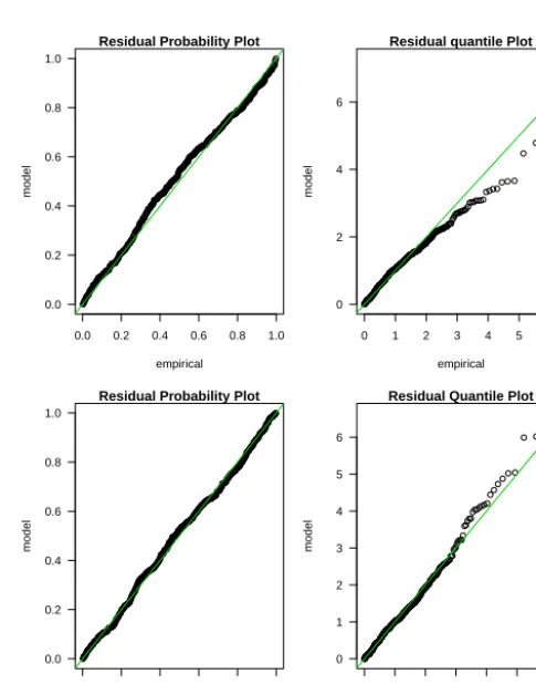
Fig. 3.Probability and quantile plots of the declustered precipitation data (in mm) based on a point process with homogeneous parameters (top panels), and with a seasonal cycle in the location parameters (bottom panels).
16
Figure 3. Probability and quantile plots of the declustered precip-itation data (in mm) based on a point process with homogeneous parameters (top panels), and with a seasonal cycle in the location parameters (bottom panels).
Table 4. Estimated parameters and BIC values for candidate gamma (left) and Weibull (right) models for daily precipitation intensity over the entire year at Ihtiman.
Gamma rate log(a) Weibull scale log(σ )
Intercept Ct St NAO Shape b BIC Intercept Ct St NAO Shape a BIC
−1.857 28 616.93 1.409 0.798 28 410.37
−1.834 0.169 0.219 0.751 28 483.62 1.418 −0.162 −0.214 0.808 28 305.52
−1.832 0.174 0.215 −0.057 0.752 28 312.39 1.416 −0.167 −0.211 −0.053 0.808 28 135.98
0 50 100 150 200
0 50 100 150 200 model obser v ed [mm] g g g g g g g g g g g g g g g g g g g g g g gggggggggggggggggggggggggggggggggggggggggggggggggggggggggggggggggggggggggggggggggggggggggggggggggggggggggggggggggggggggggggggggggggggggggggggggggggggggggggggggggggggggggggggggggggggggggggggggggggggggggggggggggggggggggggggggggggggggggggggggggggggggggggggggggggggggggggggggggggggggggggggggggggggggggggggggggggggggggggggggggggggg
gg g gg g g Q−Q plot
model:000 000 0.1 / location:Ihtiman
w w w w w w w w w w w w w w w w w w w w w w w w w w w w w w w w w w w w w w w w w w w w w w w w w w w w w w w w w w w w w w w w w w w w w w w w wwwwwwwwwwwwwwwwwwwwwwwwwwwwwwwwwwwwwwwwwwwwwwwwwwwwwwwwwwwwwwwwwwwwwwwwwwwwwwwwwwwwwwwwwwwwwwwwwwwwwwwwwwwwwwwwwwwwwwwwwwwwwwwwwwwwwwwwwwwwwwwwwwwwwwwwwwwwwwwwwwwwwwwwwwwwwwwwwwwwwwwwwwwwwwwwwwwwwwwwwwwwwwwwwwwwwwwwwwwwwwwwwwwwwwwwwwwwwwwwwwwwwwwwwwwwwwwwwwwwwwwwwwwwwwwwwwww
ww w ww
w w
:eibull−gamma distributions
0 50 100 150 200
0 50 100 150 200 model obser v ed [mm] g g g g g g g g g g g g g g g g g g g g g g g g g g g g g g g g g g g g g g g g g g g g g g g g g g g g g g g g g g g g g g g g g g g g g g g g g g g g g g g g g g g g g g g g g g g g g g g g g g g g g g g g g g g g g g g g g g g g g g g g g g g g g g g g g g g g g g g g g g g g g g g g g g g g g g g g g g g g g g g g g g g g g g g g g g g g g g g g g g g g g g g g g g g g g g g g g g g g g g g g g g g g g g g g g g g g g g g g g g g g g g g g g g g g g g g g g g g g g g g g g g g g g g g g g g g g g g g g g g g g g g g g g g g g g g g g g g g g g g g g g g g g g g g g g g g g g g g g g g g g g g g g g g g g g g g g g g g g g g g g g g g g g g g g g g g g g g g g g g g g g g g g g g g g g g g g g g g g g g g g g g g g g g g g g g g g g g g g g g g g g g g g g g g g g g g g g g g g g g g g g g g g g g g g g g g g g g g g g g g g g g g g g g g g g g g g g g g g g g g g g g g g g g g g g g g g g g g g g g g g g g g g g g g g g g g g g g g g g g g g g g g g g g g g g g g g g g g g g g g g g g g g g g g g g g g g g g g g g g g g g g g g g g g g g g g g g g g g g g g g g g g g g g g g g g g g g g g g g g g g g g g g g g g g g g g g g g g g g g g g g g g g g g g g g g g g g g g g g g g g g g g g g g g g g g g g g g g g g g g g g g g g g g g g g g g g g g g g g g g g g g g g g g g g g g g g g g g g g g g g g g g g g g g g g g g g g g g g g g g g g g g g g g g g g g g g g g g g g g g g g g g g g g g g g g g g g g g g g g g g g g g g g g g g g g g g g g g g g g g g g g g g g g g g g g g g g g g g g g g g g g g g g g g g g g g g g g g g g g g g g g g g g g g g g g g g g g g g g g g g g g g g g g g g g g g g g g g g g g g g g g g g g g g g g g g g g g g g g g g g g g g g g g g g g g g g g g g g g g g g g g g g g g g g g g g g g g g g g g g g g g g g g g g g g g g g g g g g g g g g g g g g g g g g g g g g g g g g g g g g g g g g g g g g g g g g g g g g g g g g g g g g g g g g g g g g g g g g g g g g g g g g g g g g g g g g g g g g g g g g g g g g g g g g g g g g g g g g g g g g g g g g g g g g g g g g g g g g g g g g g g g g g g g g g g g g g g g g g g g g g g g g g g g g g g g g g g g g g g g g g g g g g g g g g g g g g g g g g g g g g g g g g g g g g g g g g g g g g g g g g g g g g g g g g g g g g g g g g g g g g g g g g g g g g g g g g g g g g g g g g g g g g g g g g g g g g g g g g g g g g g g g g g g g g g g g g g g g g g g g g g g g g g g g g g g g g g g g g g g g g g g g g g g g g g g g g g g g g g g g g g g g g g g g g g g g g g g g g g g g g g g g g g g g g g g g g g g g g g g g g g g g g g g g g g g g g g g g g g g g g g g g g g g g g g g g g g g g g g g g g g g g g g g g g g g g g g g g g g g g g g g g g g g g g g g g g g g g g g g g g g g g g g g g g g g g g g g g g g g g g g g g g g g g g g g g g g g g g g g g g g g g g g ggggggggggggggggggggggggggggggggggggggggggggggggggggggggggggggggggggggggggggggggggggggggggggggggggggggggggggggggggggggggggggggggggggggggggggggggggggggggggggggggggggggggggggggggggggggggggggggggggggggggggggggggggggggggggggggggggggggggggggggggggggggggggggggggggggggggggggggggggggggggggggggggggggggggggggggggggggggggggggggggggggggggggggggggggggggggggggggggggggggggggggggggggggggggggggggggggggggggggggggggggggggggggggggggggggggggggggggggggggggggggggggggggggggggggggggggggggggggggggggggggggggggggggggggggggggggggggggggggggggggggggggggggggggggggggggggggggggggggggggggggggggggggggggggggggggggggggggggggggggggggggggggggggggggggggggggggggggggggggggggggggggggggggggggggggggggggggggggggggggggggggggggggggggggggggggggggggggggggggggggggggggggggggggggggggggggggggggggggggggggggggggggggggggggggggggggggggggggggggggggggggggggggggggggggggggggggggggggggggggggggggggggggggggggggggggggggggggggggggggggggggggggggggggggggggggggggggggggggggggggggggggggggggggggggggggggggggggggggggggggggggggggggggggggggggggggggggggggggggggggggggggggggggggggggggggggggggggggggggggggggggggggggggggggggggggggggggggggggggggggggggggggggggggggggggggggggggggggggggggggggggggggggggggggggggggggggggggggggggggggggggggggggggggggggggggggggggggggggggggggggggggggggggggggggggggggggggggggggggggggggggggggggggggggggggggggggggggggggggggggggggggggggggggggggggggggggggggggggggggggggggggggggggggggggggggggggggggggggggggggggggggggggggggggggggggggggggggggggggggggggggggggggggggggggggggggggggggggggggggggggggggggggggggggggggggggggggggggggggggggggggggggggggggggggggggggggggggggggggggggggggggggggggggggggggggggggggggggggggggggggggggggggggggggggggggggggggggggggggggggggggggggggggggggggggggggggggggggggggggggggggggggggggggggggggggggggggggggggggggggggggggggggggggggggggggggggggggggggggggggggggggggggggggggggggggggggggggggggggggggggggggggggggggggggggggggggggggggggggggggggggggggggggggggggggggggggggggggggggggggggggggggggggggggggggggggggggggggggggggggggggggggggggggggggggggggggggggggggggggggggggggggggggggggggggggggggggggggggggggggggggggggggggggggggggggggggggggggggggggggggggggggggggggggggggggggggggggggggggggggggggggggggggggggggggggggggggggggggggggggggggggggggggggggggggggggggggggggggggggggggggggggggggggggggggggggggggggggggggggggggggggggggggggggggggggggggggggggggggggggggggggggggggggggggggggggggggggggggggggggggggggggggggggggggggggggggggggggggggggggggggggggggggggggggggggggggggggggggggggggggggggggggggggggggggggggggggggggggggggggggggggggggggggggggggggggggggggggggggggggggggggggggggggggggggggggggggggggggggggggggggggggggggggggggggggggggggggggggggggggggggggggggggggggggggggggggggggggggggggggggggggggggggggggggggggggggggggggggggggggggggggggggggggggggggggggggggggggggggggggggggggggggggggggggggggggggggggggggggggggggggggggggggggggggggggggggggggggggggggggggggggggggggggggggggggggggggggggggggggggggggggggggggggggggggggggggggggggggggggggggggggggggggggggggggggggggggggggggggggggggggggggggggggggggggggggggggggggggggggggggggggggggggggggggggggggggggggggggggggggggggggggggggggggggggggggggggggggggggggggggggggggggggggggggggggggggggggggggggggggggggggggggggggggggggggggggggggggggggggggggggggggggggggggggggggggggggggggggggggggggggggggggggggggggggggggggggggggggggggggggggggggggggggggggggggggggggggggggggggggggggggggggggggggggggggggggggggggggggggggggggggggggggggggggggggggggggggggggggggggggggggggggggggggggggggggggggggggggggggggggggggggggggggggggggggggggggggggggggggggggggggggggggggggggggggggggggggggggggggggggggggggggggggggggggggggggggggggggggggggggggggggggggggggggggggggggggggggggggggggggggggggggggggggggggggggggggggggggggggggggggggggggggggggggggggggggggggggggggggggggggggggggggggggggggggggggggggggggggggggggggggggggggggggggggggggggggggggggggggggggggggggggggggggggggggggggggggggggggggggggggggggggggggggggggggggggggggggggggggggggggggggggggggggggggggggggggggggggggggggggggggggggggggggggggggggggggggggggggggggggggggggggggggggggggggggggggggggggggggggggggggggggggggggggggggggggggggggggggggggggggggggggggggggggggggggggggggggggggggggggggggggggggggggggggggggggggggggggggggggggggggggggggggggggggggggggggggggggggggggggggggggggggggggggggggggggggggggggggggggggggggggggggggggggggggggggggggggggggggggggggggggggggggggggggggggggggggggggggggggggggggggggggggggggggggggggggggggggggggggggggggggggggggggggggggggggggggggggggggggggggggggggggggggggggggggggggggggggggggggggggggggggggggggggggggggggggggggggggggggggggggggggggggggggggggggggggggggggggggggggggggggggggggggggggggggggggggggggggggggggggg
gg gg g g g Q−Q plot
model:000 000 0.1 / location:Ihtiman
w w w w w w w w w w w w w w w w w w w w w w w w w w w w w w w w w w w w w w w w w w w w w w w w w w w w w w w w w w w w w w w w w w w w w w w w w w w w w w w w w w w w w w w w w w w w w w w w w w w w w w w w w w w w w w w w w w w w w w w w w w w w w w w w w w w w w w w w w w w w w w w w w w w w w w w w w w w w w w w w w w w w w w w w w w w w w w w w w w w w w w w w w w w w w w w w w w w w w w w w w w w w w w w w w w w w w w w w w w w w w w w w w w w w w w w w w w w w w w w w w w w w w w w w w w w w w w w w w w w w w w w w w w w w w w w w w w w w w w w w w w w w w w w w w w w w w w w w w w w w w w w w w w w w w w w w w w w w w w w w w w w w w w w w w w w w w w w w w w w w w w w w w w w w w w w w w w w w w w w w w w w w w w w w w w w w w w w w w w w w w w w w w w w w w w w w w w w w w w w w w w w w w w w w w w w w w w w w w w w w w w w w w w w w w w w w w w w w w w w w w w w w w w w w w w w w w w w w w w w w w w w w w w w w w w w w w w w w w w w w w w w w w w w w w w w w w w w w w w w w w w w w w w w w w w w w w w w w w w w w w w w w w w w w w w w w w w w w w w w w w w w w w w w w w w w w w w w w w w w w w w w w w w w w w w w w w w w w w w w w w w w w w w w w w w w w w w w w w w w w w w w w w w w w w w w w w w w w w w w w w w w w w w w w w w w w w w w w w w w w w w w w w w w w w w w w w w w w w w w w w w w w w w w w w w w w w w w w w w w w w w w w w w w w w w w w w w w w w w w w w w w w w w w w w w w w w w w w w w w w w w w w w w w w w w w w w w w w w w w w w w w w w w w w w w w w w w w w w w w w w w w w w w w w w w w w w w w w w w w w w w w w w w w w w w w w w w w w w w w w w w w w w w w w w w w w w w w w w w w w w w w w w w w w w w w w w w w w w w w w w w w w w w w w w w w w w w w w w w w w w w w w w w w w w w w w w w w w w w w w w w w w w w w w w w w w w w w w w w w w w w w w w w w w w w w w w w w w w w w w w w w w w w w w w w w w w w w w w w w w w w w w w w w w w w w w w w w w w w w w w w w w w w w w w w w w w w w w w w w w w w w w w w w w w w w w w w w w wwwwwwwwwwwwwwwwwwwwwwwwwwwwwwwwwwwwwwwwwwwwwwwwwwwwwwwwwwwwwwwwwwwwwwwwwwwwwwwwwwwwwwwwwwwwwwwwwwwwwwwwwwwwwwwwwwwwwwwwwwwwwwwwwwwwwwwwwwwwwwwwwwwwwwwwwwwwwwwwwwwwwwwwwwwwwwwwwwwwwwwwwwwwwwwwwwwwwwwwwwwwwwwwwwwwwwwwwwwwwwwwwwwwwwwwwwwwwwwwwwwwwwwwwwwwwwwwwwwwwwwwwwwwwwwwwwwwwwwwwwwwwwwwwwwwwwwwwwwwwwwwwwwwwwwwwwwwwwwwwwwwwwwwwwwwwwwwwwwwwwwwwwwwwwwwwwwwwwwwwwwwwwwwwwwwwwwwwwwwwwwwwwwwwwwwwwwwwwwwwwwwwwwwwwwwwwwwwwwwwwwwwwwwwwwwwwwwwwwwwwwwwwwwwwwwwwwwwwwwwwwwwwwwwwwwwwwwwwwwwwwwwwwwwwwwwwwwwwwwwwwwwwwwwwwwwwwwwwwwwwwwwwwwwwwwwwwwwwwwwwwwwwwwwwwwwwwwwwwwwwwwwwwwwwwwwwwwwwwwwwwwwwwwwwwwwwwwwwwwwwwwwwwwwwwwwwwwwwwwwwwwwwwwwwwwwwwwwwwwwwwwwwwwwwwwwwwwwwwwwwwwwwwwwwwwwwwwwwwwwwwwwwwwwwwwwwwwwwwwwwwwwwwwwwwwwwwwwwwwwwwwwwwwwwwwwwwwwwwwwwwwwwwwwwwwwwwwwwwwwwwwwwwwwwwwwwwwwwwwwwwwwwwwwwwwwwwwwwwwwwwwwwwwwwwwwwwwwwwwwwwwwwwwwwwwwwwwwwwwwwwwwwwwwwwwwwwwwwwwwwwwwwwwwwwwwwwwwwwwwwwwwwwwwwwwwwwwwwwwwwwwwwwwwwwwwwwwwwwwwwwwwwwwwwwwwwwwwwwwwwwwwwwwwwwwwwwwwwwwwwwwwwwwwwwwwwwwwwwwwwwwwwwwwwwwwwwwwwwwwwwwwwwwwwwwwwwwwwwwwwwwwwwwwwwwwwwwwwwwwwwwwwwwwwwwwwwwwwwwwwwwwwwwwwwwwwwwwwwwwwwwwwwwwwwwwwwwwwwwwwwwwwwwwwwwwwwwwwwwwwwwwwwwwwwwwwwwwwwwwwwwwwwwwwwwwwwwwwwwwwwwwwwwwwwwwwwwwwwwwwwwwwwwwwwwwwwwwwwwwwwwwwwwwwwwwwwwwwwwwwwwwwwwwwwwwwwwwwwwwwwwwwwwwwwwwwwwwwwwwwwwwwwwwwwwwwwwwwwwwwwwwwwwwwwwwwwwwwwwwwwwwwwwwwwwwwwwwwwwwwwwwwwwwwwwwwwwwwwwwwwwwwwwwwwwwwwwwwwwwwwwwwwwwwwwwwwwwwwwwwwwwwwwwwwwwwwwwwwwwwwwwwwwwwwwwwwwwwwwwwwwwwwwwwwwwwwwwwwwwwwwwwwwwwwwwwwwwwwwwwwwwwwwwwwwwwwwwwwwwwwwwwwwwwwwwwwwwwwwwwwwwwwwwwwwwwwwwwwwwwwwwwwwwwwwwwwwwwwwwwwwwwwwwwwwwwwwwwwwwwwwwwwwwwwwwwwwwwwwwwwwwwwwwwwwwwwwwwwwwwwwwwwwwwwwwwwwwwwwwwwwwwwwwwwwwwwwwwwwwwwwwwwwwwwwwwwwwwwwwwwwwwwwwwwwwwwwwwwwwwwwwwwwwwwwwwwwwwwwwwwwwwwwwwwwwwwwwwwwwwwwwwwwwwwwwwwwwwwwwwwwwwwwwwwwwwwwwwwwwwwwwwwwwwwwwwwwwwwwwwwwwwwwwwwwwwwwwwwwwwwwwwwwwwwwwwwwwwwwwwwwwwwwwwwwwwwwwwwwwwwwwwwwwwwwwwwwwwwwwwwwwwwwwwwwwwwwwwwwwwwwwwwwwwwwwwwwwwwwwwwwwwwwwwwwwwwwwwwwwwwwwwwwwwwwwwwwwwwwwwwwwwwwwwwwwwwwwwwwwwwwwwwwwwwwwwwwwwwwwwwwwwwwwwwwwwwwwwwwwwwwwwwwwwwwwwwwwwwwwwwwwwwwwwwwwwwwwwwwwwwwwwwwwwwwwwwwwwwwwwwwwwwwwwwwwwwwwwwwwwwwwwwwwwwwwwwwwwwwwwwwwwwwwwwwwwwwwwwwwwwwwwwwwwwwwwwwwwwwwwwwwwwwwwwwwwwwwwwwwwwwwwwwwwwwwwwwwwwwwwwwwwwwwwwwwwwwwwwwwwwwwwwwwwwwwwwwwwwwwwwwwwwwwwwwwwwwwwwwwwwwwwwwwwwwwwwwwwwwwwwwwwwwwwwwwwwwwwwwwwwwwwwwwwwwwwwwwwwwwwwwwwwwwwwwwwwwwwwwwwwwwwwwwwwwwwwwwwwwwwwwwwwwwwwwwwwwwwwwwwwwwwwwwwwwwwwwwwwwwwwwwwwwwwwwwwwwwwwwwwwwwwwwwwwwwwwwwwwwwwwwwwwwwwwwwwwwwwwwwwwwwwwwwwwwwwwwwwwwwwwwwwwwwwwwwwwwwwwwwwwwwwwwwwwwwwwwwwwwwwwwwwwwwwwwwwwwwwwwwwwwwwwwwwwwwwwwwwwwwwwwwwwwwwwwwwwwwwwwwwwwwwwwwwwwwwwwwwwwwwwwwwwwwwwwwwwwwwwwwwwwwwwwwwwwwwwwwwwwwwwwwwwwwwwwwwwwwwwwwwwwwwwwwwwwwwwwwwwwwwwwwwwwwwwwwwwwwwwwwwwwwwwwwwwwwwwwwwwwwwwwwwwwwwwwwwwwwwwwwwwwwwwwwwwwwwwwwwwwwwwwwwwwwwwwwwwwwwwwwwwwwwwwwwwwwwwwwwwwwwwwwwwwwwwwwwwwwwwwwwwwwwwwwwwwwwwwwwwwwwwwwwwwwwwwwwwwwwwwwwwwwwwwwwwwwwwwwwwwwwwwwwwwwwwwwwwwwwwwwwwwwwwwwwwwwwwwwwwwwwwwwwwwwwwwwwwwwwwwwwwwwwwwwwwwwwwwwwwwwwwwwwwwwwwwwwwwwwwwwwwwwwwwwwwwwwwwwwwwwwwwwwwwwwwwwwwwwwwwwwwwwwwwwwwwwwwwwwwwwwwwwwwwwwwwwwwwwwwwwwwwwwwwwwwwwwwwwwwwwwwwwwwwwwwwwwwwwwwwwwwwwwwwwwwwwwwwwwwwwwwwwwwwwwwwwwwwwwwwwwwwwwwwwwwwwwwwwwwwwwwwwwwwwwwwwwwwwwwwwwwwwwwwwwwwwwwwwwwwwwwwwwwwwwwwwwwwwwwwwwwwwwwwwwwwwwwwwwwwwwwwwwwwwwwwwwwwwwwwwwwwwwwwwwwwwwwwwwwwwwwwwwwwwwwwwwwwwwwwwwwwwwwwwwwwwwwwwwwwwwwwwwwwwwwwwwwwwwwwwwwwwwwwwwwwwwwwwwwwwwwwwwwwwwwwwwwwwwwwwwwwwwwwwwwwwwwwwwwwwwwwwwwwwwwwwwwwwwwwwwwwwwwwwwwwwwwwwwwwwwwwwwwwwwwwwwwwwwwwwwwwwwwwwwwwwwwwwwwwwwwwwwwwwwwwwwwwwwwwwwwwwwwwwwwwwwwwwwwwwwwwwwwwwwwwwwwwwwwwwwwwwwwwwwwwwwwwwwwwwwwwwwwwwwwwwwwwwwwwwwwwwwwwwwwwwwwwwwwwwwwwwwwwwwwwwwwwwwwwwwwwwwwwwwwwwwwwwwwwwwwwwwwwwwwwwwwwwwwwwwwwwwwwwwwwwwwwwwwwwwwwwwwwwwwwwwwwwwwwwwwwwwwwwwwwwwwwwwwwwwwwwwwwwwwwwwwwwwwwwwwwwwwwwwwwwwwwwwwwwwwwwwwwwwwwwwwwwwwwwwwwwwwwwwwwwwwwwwwwwwwwwwwwwwwwwwwwwwwwwwwwwwwwwwwwwwwwwwwwwwwwwwwwwwwwwwwwwwwwwwwwwwwwwwwwwwwwwwwwwwwwwwwwwwwwwwwwwwwwwwwwwwwwwwwwwwwwwwwwwwwwwwwwwwwwwwwwwwwwwwwwwwwwwwwwwwwwwwwwwwwwwwwwwwwwwwwwwwwwwwwwwwwwwwwwwwwwwwwwwwwwwwwwwwwwwwwwwwwwwwwwwwwwwwwwwwwwwwwwwwwwwwwwwwwwwwwwwwwwwwwwwwwwwwwwwwwwwwwwwwwwwwwwwwwwwwwwwwwwwwwwwwwwwwwwwwwwwwwwwwwwwwwwwwwwwwwwwwwwwwwwwwwwwwwwwwwwwwwwwwwwwwwwwwwwwwwwwwwwwwwwwwwwwwwwwwwwwwwwwwwwwwwwwwwwwwwwwwwwwwwwwwwwwwwwwwwwwwwwwwwwwwwwwwwwwwwwwwwwwwwwwwwwwwwwwwwwwwwwwwwwwwwwwwwwwwwwwwwwwwwwwwwwwwwwwwwwwwwwwwwwwwwwwwwwwwwwwwwwwwwwwwwwwwwwwwwwwwwwwwwwwwwwwwwwwwwwwwwwwwwwwwwwwwwwwwwwwwwwwwwwwwwwwwwwwwwwwwwwwwwwwwwwwwwwwwwwwwwwwwwwwwwwwwwwwwwwwwwwwwwwwwwwwwwwwwwwwwwwwwwwwwwwwwwwwwwwwwwwwwwwwwwwwwwwwwwwwwwwwwwwwwwwwwwwwwwwwwwwwwwwwwwwwwwwwwwwwwwwwwwwwwwwwwwwwwwwwwwwwwwwwwwwwwwwwwwwwwwwwwwwwwwwwwwwwwwwwwwwwwwwwwwwwwwwwwwwwwwwwwwwwwwwwwwwwwwwwwwwwwwwwwwwwwwwwwwwwwwwwwwwwwwwwwwwwww
ww ww
w w
w
:eibull−gamma distributions
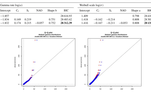
Fig. 4.Q-Q plots of observed versus fitted gamma (g) and Weibull (w) quantiles of daily precipitation intensities
(standard threshold of 0.1 mm) based on homogeneous model in August (left plot) and for the entire year (right plot).
0 50 100 150 200
−40 −30 −20 −10 0 Precipitation [mm] log density
Log−density of hybrid distribution gamma/GP distribution model:000 000 5 / location:Ihtiman
gamma GP gamma−hybrid GP−hybrid
0 50 100 150 200
−40 −30 −20 −10 0 Precipitation [mm] log density
Log−density of hybrid distribution gamma/GP distribution model:000 000 10 / location:Ihtiman
gamma GP gamma−hybrid GP−hybrid
0 50 100 150 200
−40 −30 −20 −10 0 Precipitation [mm] log density
Log−density of hybrid distribution gamma/GP distribution model:000 000 20 / location:Ihtiman
gamma GP gamma−hybrid GP−hybrid
0 50 100 150 200
−25 −20 −15 −10 −5 0 Precipitation [mm] log density
Log−density of hybrid distribution weibull/GP distribution model:000 000 5 / location:Ihtiman
weibull GP weibull−hybrid GP−hybrid
0 50 100 150 200
−25 −20 −15 −10 −5 0 Precipitation [mm] log density
Log−density of hybrid distribution weibull/GP distribution model:000 000 10 / location:Ihtiman
weibull GP weibull−hybrid GP−hybrid
0 50 100 150 200
−25 −20 −15 −10 −5 0 Precipitation [mm] log density
Log−density of hybrid distribution weibull/GP distribution model:000 000 20 / location:Ihtiman
weibull GP weibull−hybrid GP−hybrid
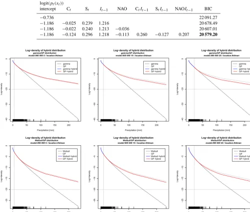
Fig. 5. Top panels: log-density functions fitted to daily precipitation intensity with threshold values 5 mm, 10
mm and 20 mm. Gamma (solid and dashed lines), GP (dotted lines) and hybrid gamma–GP (solid blue and
red lines) models are shown. The data are indicated by horizontal ticks and the thresholduby a vertical line.
Bottom line: The same as the top row but based on the Weibull and hybrid Weibull–GP distributions.
17
Figure 4. Q–Q plots of observed versus fitted gamma (g) and Weibull (w) quantiles of daily precipitation intensities (standard threshold of
0.1 mm), based on a homogeneous model in August (left plot) and for the entire year (right plot).
of thresholds for which the resulting GP distribution param-eter estimates do not change considerably, and at the same time, the fit provides a reasonable model approximation; see the next paragraph for details. We note that the time-varying threshold is a continuous analog of the widely used proce-dure of splitting the data into seasons and allowing for differ-ent thresholds in each season. The monthly threshold values based on this model are given in Table 1.
4.2 Fitting of extreme precipitation
Having estimated the time-varying threshold model, clus-ters of exceedances separated from each other by 3-day run length are identified, and each cluster maximum is selected. This is done to avoid dependence in the likelihood specifi-cation. In this way, 557 peaks out of 17 532 observations were extracted, resulting in a rate of 11.60 in excesses per year. The cluster peaks are displayed in the right panel of Fig. 2. The tiny black bullets and circles correspond to cold-and warm-month intensities, respectively. This plot exhibits higher precipitation intensities during the warmer months. These extreme intensities are fitted using a point process model, as in Coles (2001). The advantage of the point process approach is that it unifies the classical block maxima (GEV)
and peaks over threshold (GP distribution) approaches, and allows modeling of the location, scale and shape parame-ters of the GEV distributions as functions of time-dependent covariates in order to account for non-stationarity effects. The parameter estimates and Bayesian information criterion (BIC) values for several model fits are presented in Table 2. The main message from the results of this table is that the distribution of the extreme precipitation intensity at station Ihtiman has a heavy tail. This is supported by the likeli-hood ratio test (LRT) concerning the hypothesisξ =0 (ex-ponential distribution) versusξ >0 (GP distribution); for all models, the corresponding tail probability is quite small. We note that not all precipitation data series over the territory of Bulgaria exhibit heavy upper tails, especially for sites with relatively short records. This is in agreement with the main conclusions of Papalexiou et al. (2013). The non-stationary model that minimizes the BIC includes a seasonal cycle and a lagged NAO effect in the location parameter, and a sea-sonal cycle in the (logarithm of the) scale parameter, and has a constant shape parameter. The estimated parameters of this model support the notion that higher location val-ues are associated with higher precipitation intensities syn-chronized with negative NAO index anomalies. On the other hand, higher scale parameter estimates are associated with
N. M. Neykovet al.: Stochastic daily precipitation model with a heavy-tailed component 2327
Table 5. Estimated parameters and BIC values for daily precipitation occurrence models over the entire year at Ihtiman.
logit(pt(xt))
intercept Ct St It−1 NAO CtIt−1 StIt−1 NAOIt−1 BIC
−0.736 22 091.27
−1.186 −0.025 0.239 1.216 20 678.49
−1.186 −0.022 0.240 1.213 −0.036 20 607.01
−1.186 −0.124 0.296 1.218 −0.113 0.260 −0.127 0.207 20 579.20
0 50 100 150 200
−40
−30
−20
−10
0
Precipitation [mm]
Log
−
density
Log−density of hybrid distribution
gamma/GP distribution model:000 000 5 / location:Ihtiman
gamma GP gamma−hybrid GP−hybrid
0 50 100 150 200
−40
−30
−20
−10
0
Precipitation [mm]
Log
−
density
Log−density of hybrid distribution
gamma/GP distribution model:000 000 10 / location:Ihtiman
gamma GP gamma−hybrid GP−hybrid
0 50 100 150 200
−40
−30
−20
−10
0
Precipitation [mm]
Log
−
density
Log−density of hybrid distribution
gamma/GP distribution model:000 000 20 / location:Ihtiman
gamma GP gamma−hybrid GP−hybrid
0 50 100 150 200
−2
5
−2
0
−1
5
−1
0
−
5
0
Precipitation [mm]
Log
−
density
Log−density of hybrid distribution
Weibull/GP distribution model:000 000 5 / location:Ihtiman
Weibull GP Weibull−hybrid GP−hybrid
0 50 100 150 200
−2
5
−2
0
−1
5
−1
0
−
5
0
Precipitation [mm]
Log
−
density
Log−density of hybrid distribution
Weibull/GP distribution model:000 000 10 / location:Ihtiman
Weibull GP Weibull−hybrid GP−hybrid
0 50 100 150 200
−2
5
−2
0
−1
5
−1
0
−
5
0
Precipitation [mm]
Log
−
density
Log−density of hybrid distribution
Weibull/GP distribution model:000 000 20 / location:Ihtiman
Weibull GP Weibull−hybrid GP−hybrid
Figure 5. Top panels: log-density functions fitted to daily precipitation intensity with threshold values 5, 10 and 20 mm. Gamma (solid and dashed lines), GP (dotted lines) and hybrid gamma–GP (solid blue and red lines) models are shown. The data are indicated by horizontal ticks,
and the thresholduby a vertical line. Bottom line: the same as the top row, but based on the Weibull and hybrid Weibull–GP distributions.
higher variability in precipitation extremes. The scale in-tercept estimate of this model equals exp(2.413)=11.167. Residual probability plots for the homogeneous model (with no covariates), and the best among these 6 fits (according to the BIC), are shown in Fig. 3. The plots indicate reasonable but by no means perfect fits, and that the non-stationary fits are better than the homogeneous model. The corresponding return levels are given in Table 3. It is seen that the non-stationary model gives reasonable return-level estimates for the historical data. All the computations in this section were
done by the pp.fit and pp.diag procedures from R package ismev.
4.3 Gamma and Weibull intensity models
In this section, we compare a number of simple gamma and Weibull models with and without covariates (seasonal cycle and NAO effect), in order to assess their ability to fit the entire intensity series. Each model can be identified by its unique abbreviation code “xxx yyy zz” at the top of the in-dividual panel of the corresponding figure. The strings xxx, yyy and zz indicate the occurrence, intensity and threshold
0 100 200 300
0
20
40
60
80
100
120
140
day of year
95%,99% quantile [mm]
High quantiles
gamma/GP distribution model:100 100 5 / location:Ihtiman
observed 99% hybrid 95% hybrid 99% gamma 95% gamma
0 100 200 300
20
40
60
80
100
120
140
day of year
95%,99% quantile [mm]
High quantiles
gamma/GP distribution model:100 100 15 / location:Ihtiman
observed 99% hybrid 95% hybrid 99% gamma 95% gamma
0 100 200 300
0
20
40
60
80
100
120
140
day of year
95%,99% quantile [mm]
High quantiles
:eibull/GP distribution model:100 100 5 / location:Ihtiman
observed 99% hybrid 95% hybrid 99% weibull 95% weibull
0 100 200 300
20
40
60
80
100
120
140
day of year
95%,99% quantile [mm]
High quantiles
:eibull/GP distribution model:100 100 15 / location:Ihtiman
observed 99% hybrid 95% hybrid 99% weibull 95% weibull
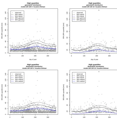
Fig. 6. Top row: High quantiles (95% and 99%) of fitted gamma (solid lines) and hybrid gamma–GP (dashed
lines) distributions as functions of the day of the year for Ihtiman precipitation intensity with thresholds 5mm
(left) and 15 mm (right). Lower line plots: The same as the top row but based on Weibull and hybrid Weibull– GP distributions.
18
Figure 6. Top row: high quantiles (95 and 99 %) of fitted gamma (solid lines) and hybrid gamma–GP (dashed lines) distributions as functions of the day of the year for Ihtiman precipitation intensity with thresholds 5 mm (left) and 15 mm (right). Lower-line plots: the same as the top row, but based on Weibull and hybrid Weibull–GP distributions.
value model components, respectively. The coding depends on the types of covariates in the model components. For instance, (i) the model without covariates (homogeneous model) is coded as 000 000, (ii) the model with sine and co-sine waves and previous day occurrence is coded as 100 100, and (iii) the model (ii) with additional lag of the NAO effect is coded as 110 110. This way, we get various gamma and Weibull precipitation models.
The corresponding parameter estimates and BIC values are given in Table 4. The homogeneous models are presented for completeness only. It is seen that the inclusion of a peri-odic component significantly reduces the BIC values of both the gamma and Weibull models. According to the LRT, the models with seasonal components lead to improvements in comparison with homogeneous models, and the inclusion of NAO effects leads to further improvements. (The LRT and
its tail probability values are not presented.) Both models preserve the physical interpretation that heavier intensities are associated with negative NAO anomalies. The left plot of Fig. 4 shows a quantile–quantile (Q–Q) plot for the model, with a seasonal cycle based on the GLMs with gamma and Weibull fits. The left panel of the figure is based on data for a single month (August), whereas the right panel is for the entire period. The Weibull distribution leads to a slightly bet-ter fit, but the fits are poor with respect to extreme intensities. For validation purposes, the parameter estimates of some simple daily precipitation occurrence models are presented in Table 5. Obviously, the homogeneous model is completely inadequate, but one can see the BIC value reduction, with the remaining models conditional on seasonal cycle, previous day precipitation occurrence and NAO effect with lag one.
N. M. Neykovet al.: Stochastic daily precipitation model with a heavy-tailed component 2329
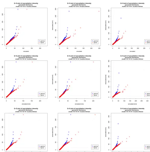
Figure 7. Q–Q plots of simulated versus observed gamma (g) and hybrid gamma–GP (h) quantiles of intensity seasonal models with the
NAO effect for the entire year at Ihtiman, with 5 mm (top row), 10 mm (middle row) and 15 mm (bottom row) thresholds.
Figure 8. Monthly boxplots of daily observed and simulated precipitation totals in log scale. The simulated data are generated using a seasonal model with a lagged NAO covariate; the intensity component is based on (i) hybrid gamma–GP (top-left and middle plots) and Weibull–GP (bottom-left and middle plots) distributions with threshold values 5 and 15 mm, and (ii) standard gamma and Weibull distributions (right-column plots).
As expected, the seasonal model with lagged occurrence and NAO effects minimizes the BIC.
5 Hybrid gamma–GP density
Furrer and Katz (2008) define the density function of the hy-brid gamma–GP distribution as
h(x)=
(
f (x) x≤u
(1−F (u))g(x) x > u,
where F (x) is the gamma distribution function, f (x) and
g(x) are the gamma and GP densities, and the factor (1−
F (u))ensuresh(x)normalization.
In order to attain continuity at the thresholdu, these au-thors impose the condition
f (u)= [1−F (u)]g(u)= [1−F (u)]/σ.
The resulting GP distribution scale parameter is equal to
σ =(1−F (u))/f (u), which is the inverse of the hazard
func-tion of the gamma distribufunc-tion taken atu. The GP distribution
scale parameter can thus be written in terms of the parame-ters of the gamma distribution that accommodates the ob-servations below the threshold. The authors recommend the following estimation procedure: (i) fit a GLMs with a gamma link function with covariates to the entire intensity data set; (ii) fit a GP distribution with covariates to the observations above the prespecified threshold u, just as in the conven-tional extreme value methodology; and (iii) replace the GP distribution scale parameter with the estimated gamma haz-ard function. Clearly, an analogous procedure is applicable for other hybrid distributions, such as Weibull–GP or inverse Gaussian–GP.
5.1 Experiments with hybrid GP distributions
As in the previous section, the models discussed hereafter can be identified by their unique code. However, gamma and Weibull intensity model components are combined with the GP distribution at the prespecified threshold values, e.g., 5, 10 and 15 mm. This way, we consider several hybrid gamma– GP and Weibull–GP distribution models. We now compare
N. M. Neykovet al.: Stochastic daily precipitation model with a heavy-tailed component 2331
the fit of these models to Ihtiman daily precipitation inten-sity data. We explore the threshold selection and its effect on generation of artificial daily precipitation data. The method-ology of Furrer and Katz (2008) previously described is fol-lowed closely.
Figure 5 shows the fitted gamma, GP, and hybrid gamma– GP (upper-line plots), and Weibull, GP and Weibull–GP (lower-line plots) log densities, with three threshold values 5, 10 and 20 mm for precipitation intensity for the entire year. The homogeneous fits (no covariates in the model) are shown only in order to get a better perception. The hybrid density is indeed continuous, and possesses a heavier tail than the gamma and Weibull densities. One can see the effect of the threshold choice in GP distribution tail estimation. A lower threshold choice u gives a larger weight, 1−F (u), of the GP distribution. One can thus expect that the hybrid distri-bution quantiles corresponding to these lower-threshold GP fits would be larger. The plots of Fig. 6 show the 95 % (blue) and 99 % (black) quantiles of the fitted gamma (solid lines) and hybrid gamma–GP (dashed lines) distributions (upper-line plots), as well as the fitted Weibull and hybrid Weibull– GP (lower-line plots) distributions as functions of the day of the year. The tiny black bullets in the plots correspond to ob-served precipitation totals exceeding the prespecified thresh-old. Indeed, the hybrid quantiles (dashed lines) in the left-column plots are higher than those in the right-left-column plots. The effect due to hybridization is most visible in the high-est quantiles. Therefore, threshold determination is of crucial importance to calibration daily precipitation hybrid models, conditional on atmospheric covariates.
Figure 7 shows Q–Q plots of observed versus simulated gamma (g) and hybrid gamma–GP (h) quantiles of the sea-sonal intensity model with a lagged NAO effect over a year at Ihtiman, with 5 mm (top row), 10 mm (middle row) and 15 mm (bottom row) thresholds. The simulated time series consist of 300 samples of 47 yr of daily precipitation totals from GLMs, with the gamma distribution (g) and with the gamma–GP (h) hybrid distributions for each threshold. The majority of the simulated data look like those displayed in the left and middle column plots, but a small percentage look like those displayed in the right column plots. Results of a similar standard are obtained for the Weibull and Weibull–GP dis-tributions. The hybrid models are a significant improvement over the gamma and Weibull models.
The monthly boxplots of daily observed (white) and sim-ulated (gray) precipitation totals given on logarithmic scales are presented in the plots of Fig. 8 in order to get an impres-sion of their distributions: the left and middle column panels are based on the hybrid intensity distributions, with 5 and 15 mm thresholds where the right column panels are based on classical GLMs with the gamma and Weibull distribu-tions. The classical GLMs with gamma and Weibull intensity components represent the historical data, except for the ex-treme intensities, which is a well known deficiency. The hy-brid models are capable of generating series with extremes as
large as the observed extremes, or (though unlikely to occur) even larger, depending on the threshold choice. The distri-butions of the monthly observed and simulated precipitation totals are presented in the plots of Fig. 9. From the right-column plots of this figure, one can see that the standard-intensity GLMs with the gamma and Weibull distributions are not capable of generating monthly precipitation totals with similar magnitudes as the historical ones, whereas the hybrid gamma and Weibull–GP distributions are capable of doing so. The distribution functions of the wet spells and the number of wet days within a season are important in applica-tions in various studies. The left plot of Fig. 10 shows the dis-tribution of wet spells for the historical and simulated data. As usual, wet spells are defined as the number of consecu-tive days with precipitation. It is seen that the model cap-tures well the temporal correlation in the data. The middle and right plots of this figure show the monthly number of wet days distribution of historical versus simulated data. Re-sults of a similar standard are obtained for the Weibull and Weibull–GP distributions.
The distributions of the observed (solid lines) and simu-lated (dotted lines) precipitation totals over periods of 10 and 60 days are shown in the plots of Fig. 11. The simulated data are generated using intensity GLMs with hybrid Weibull–GP distributions and a threshold of 15 mm (left-column plots), and standard Weibull (right-column plots) distributions. It is seen that the hybrid Weibull–GP distribution-simulated data possess a heavier tail than the standard Weibull distribution. Similar results are obtained for the gamma–GP hybrid distri-bution.
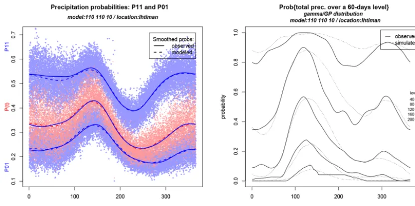
The left-plot dots of Fig. 12 show the different seasonal cycles as well as the different magnitudes of the estimated precipitation probabilitiesp11(t )andp01(t ), and the
uncon-ditional precipitation probabilityp(t ):=π(t )(red).
The dashed and smoothed lines are based on the R locally weighted scatterplot smoothing procedure loess through the corresponding dots and observed frequencies (not plotted). In the right plot of this figure are given the historical and sim-ulated probabilities (smoothed by loess) of having not less than 40, 80, 120, 160 and 200 mm total precipitation for a run of 60 consecutive days, starting on any given day of the year for Ihtiman station. The order of the lines corresponds to their order in the legend. The empirical and model probabilities match each other closely.
All model fitting and generation of precipitation series was done with the free software environment for statistical com-puting and graphics: the R Project for Statistical Comcom-puting. The vglm procedure from the VGAM package with gamma, Weibull and GP distribution link functions was used to carry out the estimation (Yee and Stephenson, 2007).
2332 N. M. Neykovet al.: Stochastic daily precipitation model with a heavy-tailed component
2 4 6 8 10 12
0 100 200 300 400 months
monthly amount [mm]
0 100 200 300 400 0 100 200 300 400 0 100 200 300 400 0 100 200 300 400 0 100 200 300 400 0 100 200 300 400 0 100 200 300 400 0 100 200 300 400 0 100 200 300 400 0 100 200 300 400 0 100 200 300 400 0 100 200 300 400 0 100 200 300 400 0 100 200 300 400 0 100 200 300 400 0 100 200 300 400 0 100 200 300 400 0 100 200 300 400 0 100 200 300 400 0 100 200 300 400 0 100 200 300 400 0 100 200 300 400 0 100 200 300 400 0 100 200 300 400
Monthly precipitation amount
gamma/GP distribution model:110 110 5 / location:Ihtiman
observed simulated
2 4 6 8 10 12
0 100 200 300 400 months
monthly amount [mm]
0 100 200 300 400 0 100 200 300 400 0 100 200 300 400 0 100 200 300 400 0 100 200 300 400 0 100 200 300 400 0 100 200 300 400 0 100 200 300 400 0 100 200 300 400 0 100 200 300 400 0 100 200 300 400 0 100 200 300 400 0 100 200 300 400 0 100 200 300 400 0 100 200 300 400 0 100 200 300 400 0 100 200 300 400 0 100 200 300 400 0 100 200 300 400 0 100 200 300 400 0 100 200 300 400 0 100 200 300 400 0 100 200 300 400 0 100 200 300 400
Monthly precipitation amount
gamma/GP distribution model:110 110 15 / location:Ihtiman
observed simulated
2 4 6 8 10 12
0 100 200 300 400 months
monthly amount [mm]
0 100 200 300 400 0 100 200 300 400 0 100 200 300 400 0 100 200 300 400 0 100 200 300 400 0 100 200 300 400 0 100 200 300 400 0 100 200 300 400 0 100 200 300 400 0 100 200 300 400 0 100 200 300 400 0 100 200 300 400 0 100 200 300 400 0 100 200 300 400 0 100 200 300 400 0 100 200 300 400 0 100 200 300 400 0 100 200 300 400 0 100 200 300 400 0 100 200 300 400 0 100 200 300 400 0 100 200 300 400 0 100 200 300 400 0 100 200 300 400
Monthly precipitation amount
gamma distribution model:110 110 0.1 / location:Ihtiman
observed simulated
2 4 6 8 10 12
0 100 200 300 400 months
monthly amount [mm]
0 100 200 300 400 0 100 200 300 400 0 100 200 300 400 0 100 200 300 400 0 100 200 300 400 0 100 200 300 400 0 100 200 300 400 0 100 200 300 400 0 100 200 300 400 0 100 200 300 400 0 100 200 300 400 0 100 200 300 400 0 100 200 300 400 0 100 200 300 400 0 100 200 300 400 0 100 200 300 400 0 100 200 300 400 0 100 200 300 400 0 100 200 300 400 0 100 200 300 400 0 100 200 300 400 0 100 200 300 400 0 100 200 300 400 0 100 200 300 400
Monthly precipitation amount :eibull/GP distribution model:110 110 5 / location:Ihtiman
observed simulated
2 4 6 8 10 12
0 100 200 300 400 months
monthly amount [mm]
0 100 200 300 400 0 100 200 300 400 0 100 200 300 400 0 100 200 300 400 0 100 200 300 400 0 100 200 300 400 0 100 200 300 400 0 100 200 300 400 0 100 200 300 400 0 100 200 300 400 0 100 200 300 400 0 100 200 300 400 0 100 200 300 400 0 100 200 300 400 0 100 200 300 400 0 100 200 300 400 0 100 200 300 400 0 100 200 300 400 0 100 200 300 400 0 100 200 300 400 0 100 200 300 400 0 100 200 300 400 0 100 200 300 400 0 100 200 300 400
Monthly precipitation amount :eibull/GP distribution model:110 110 15 / location:Ihtiman
observed simulated
2 4 6 8 10 12
0 100 200 300 400 months
monthly amount [mm]
0 100 200 300 400 0 100 200 300 400 0 100 200 300 400 0 100 200 300 400 0 100 200 300 400 0 100 200 300 400 0 100 200 300 400 0 100 200 300 400 0 100 200 300 400 0 100 200 300 400 0 100 200 300 400 0 100 200 300 400 0 100 200 300 400 0 100 200 300 400 0 100 200 300 400 0 100 200 300 400 0 100 200 300 400 0 100 200 300 400 0 100 200 300 400 0 100 200 300 400 0 100 200 300 400 0 100 200 300 400 0 100 200 300 400 0 100 200 300 400
Monthly precipitation amount :eibull distribution model:110 110 0.1 / location:Ihtiman
observed simulated
Fig. 9.
Box-plots of monthly observed and simulated precipitation totals. The simulated data are generated
using seasonal model with a lagged NAO covariate; the intensity component is based on: (i) hybrid gamma–GP
(top left and middle plots) and Weibull–GP (bottom left and middle plots) distributions with threshold values 5
mm and 15 mm; (ii) standard gamma and Weibull distributions (right column plots).
0 5 10 15
0.0 0.2 0.4 0.6 0.8 1.0 days Prob{w
et spells > da
ys}
Wet spells
gamma/GP distribution model:110 110 10 / location:Ihtiman
observed simulatted
2 4 6 8 10 12
0 5 10 15 20 25 months monthly n
umber of w
et da ys 0 5 10 15 20 25 0 5 10 15 20 25 0 5 10 15 20 25 0 5 10 15 20 25 0 5 10 15 20 25 0 5 10 15 20 25 0 5 10 15 20 25 0 5 10 15 20 25 0 5 10 15 20 25 0 5 10 15 20 25 0 5 10 15 20 25 0 5 10 15 20 25 0 5 10 15 20 25 0 5 10 15 20 25 0 5 10 15 20 25 0 5 10 15 20 25 0 5 10 15 20 25 0 5 10 15 20 25 0 5 10 15 20 25 0 5 10 15 20 25 0 5 10 15 20 25 0 5 10 15 20 25 0 5 10 15 20 25 0 5 10 15 20 25
Monthly number of days with precipitation totals > 0.1 mm
gamma/GP distribution model:110 110 15 / location:Ihtiman
observed simulatted
2 4 6 8 10 12
0 5 10 15 20 25 months monthly n
umber of w
et da ys 0 5 10 15 20 25 0 5 10 15 20 25 0 5 10 15 20 25 0 5 10 15 20 25 0 5 10 15 20 25 0 5 10 15 20 25 0 5 10 15 20 25 0 5 10 15 20 25 0 5 10 15 20 25 0 5 10 15 20 25 0 5 10 15 20 25 0 5 10 15 20 25 0 5 10 15 20 25 0 5 10 15 20 25 0 5 10 15 20 25 0 5 10 15 20 25 0 5 10 15 20 25 0 5 10 15 20 25 0 5 10 15 20 25 0 5 10 15 20 25 0 5 10 15 20 25 0 5 10 15 20 25 0 5 10 15 20 25 0 5 10 15 20 25
Monthly number of days with precipitation totals > 0.1 mm
gamma distribution model:110 110 0.1 / location:Ihtiman
observed simulatted
Fig. 10.
Left plot: observed (solid lines) and simulated (dotted lines) wet spells distribution. Box-plots of
monthly observed (white) versus simulated (gray) number of wet days: the simulated data are based on the
hybrid gamma–GP distribution with threshold 15 mm and standard gamma (right plot) distribution.
21
Figure 9. Boxplots of monthly observed and simulated precipitation totals. The simulated data are generated using a seasonal model with a lagged NAO covariate; the intensity component is based on (i) hybrid gamma–GP (top-left and middle plots) and Weibull–GP (bottom-left and middle plots) distributions with threshold values of 5 and 15 mm, and (ii) standard gamma and Weibull distributions (right-column plots).
2 4 6 8 10 12
0 100 200 300 400 months
monthly amount [mm]
0 100 200 300 400 0 100 200 300 400 0 100 200 300 400 0 100 200 300 400 0 100 200 300 400 0 100 200 300 400 0 100 200 300 400 0 100 200 300 400 0 100 200 300 400 0 100 200 300 400 0 100 200 300 400 0 100 200 300 400 0 100 200 300 400 0 100 200 300 400 0 100 200 300 400 0 100 200 300 400 0 100 200 300 400 0 100 200 300 400 0 100 200 300 400 0 100 200 300 400 0 100 200 300 400 0 100 200 300 400 0 100 200 300 400 0 100 200 300 400 observed simulatted
2 4 6 8 10 12
0 100 200 300 400 months
monthly amount [mm]
0 100 200 300 400 0 100 200 300 400 0 100 200 300 400 0 100 200 300 400 0 100 200 300 400 0 100 200 300 400 0 100 200 300 400 0 100 200 300 400 0 100 200 300 400 0 100 200 300 400 0 100 200 300 400 0 100 200 300 400 0 100 200 300 400 0 100 200 300 400 0 100 200 300 400 0 100 200 300 400 0 100 200 300 400 0 100 200 300 400 0 100 200 300 400 0 100 200 300 400 0 100 200 300 400 0 100 200 300 400 0 100 200 300 400 0 100 200 300 400 observed simulatted
2 4 6 8 10 12
0 100 200 300 400 months
monthly amount [mm]
0 100 200 300 400 0 100 200 300 400 0 100 200 300 400 0 100 200 300 400 0 100 200 300 400 0 100 200 300 400 0 100 200 300 400 0 100 200 300 400 0 100 200 300 400 0 100 200 300 400 0 100 200 300 400 0 100 200 300 400 0 100 200 300 400 0 100 200 300 400 0 100 200 300 400 0 100 200 300 400 0 100 200 300 400 0 100 200 300 400 0 100 200 300 400 0 100 200 300 400 0 100 200 300 400 0 100 200 300 400 0 100 200 300 400 0 100 200 300 400 observed simulatted
2 4 6 8 10 12
0 100 200 300 400 months
monthly amount [mm]
0 100 200 300 400 0 100 200 300 400 0 100 200 300 400 0 100 200 300 400 0 100 200 300 400 0 100 200 300 400 0 100 200 300 400 0 100 200 300 400 0 100 200 300 400 0 100 200 300 400 0 100 200 300 400 0 100 200 300 400 0 100 200 300 400 0 100 200 300 400 0 100 200 300 400 0 100 200 300 400 0 100 200 300 400 0 100 200 300 400 0 100 200 300 400 0 100 200 300 400 0 100 200 300 400 0 100 200 300 400 0 100 200 300 400 0 100 200 300 400
Monthly precipitation amount
weibull/GP distribution model:110 110 5 / location:Ihtiman
observed simulatted
2 4 6 8 10 12
0 100 200 300 400 months
monthly amount [mm]
0 100 200 300 400 0 100 200 300 400 0 100 200 300 400 0 100 200 300 400 0 100 200 300 400 0 100 200 300 400 0 100 200 300 400 0 100 200 300 400 0 100 200 300 400 0 100 200 300 400 0 100 200 300 400 0 100 200 300 400 0 100 200 300 400 0 100 200 300 400 0 100 200 300 400 0 100 200 300 400 0 100 200 300 400 0 100 200 300 400 0 100 200 300 400 0 100 200 300 400 0 100 200 300 400 0 100 200 300 400 0 100 200 300 400 0 100 200 300 400
Monthly precipitation amount
weibull/GP distribution model:110 110 15 / location:Ihtiman
observed simulatted
2 4 6 8 10 12
0 100 200 300 400 months
monthly amount [mm]
0 100 200 300 400 0 100 200 300 400 0 100 200 300 400 0 100 200 300 400 0 100 200 300 400 0 100 200 300 400 0 100 200 300 400 0 100 200 300 400 0 100 200 300 400 0 100 200 300 400 0 100 200 300 400 0 100 200 300 400 0 100 200 300 400 0 100 200 300 400 0 100 200 300 400 0 100 200 300 400 0 100 200 300 400 0 100 200 300 400 0 100 200 300 400 0 100 200 300 400 0 100 200 300 400 0 100 200 300 400 0 100 200 300 400 0 100 200 300 400
Monthly precipitation amount
weibull distribution model:110 110 0.1 / location:Ihtiman
observed simulatted
Fig. 9.
Box-plots of monthly observed and simulated precipitation totals. The simulated data are generated
using seasonal model with a lagged NAO covariate; the intensity component is based on: (i) hybrid gamma–GP
(top left and middle plots) and Weibull–GP (bottom left and middle plots) distributions with threshold values 5
mm and 15 mm; (ii) standard gamma and Weibull distributions (right column plots).
0 5 10 15
0.0 0.2 0.4 0.6 0.8 1.0 days Prob{w
et spells > da
ys}
Wet spells
gamma/GP distribution model:110 110 10 / location:Ihtiman
observed simulated
2 4 6 8 10 12
0 5 10 15 20 25 months monthly n
umber of w
et da ys 0 5 10 15 20 25 0 5 10 15 20 25 0 5 10 15 20 25 0 5 10 15 20 25 0 5 10 15 20 25 0 5 10 15 20 25 0 5 10 15 20 25 0 5 10 15 20 25 0 5 10 15 20 25 0 5 10 15 20 25 0 5 10 15 20 25 0 5 10 15 20 25 0 5 10 15 20 25 0 5 10 15 20 25 0 5 10 15 20 25 0 5 10 15 20 25 0 5 10 15 20 25 0 5 10 15 20 25 0 5 10 15 20 25 0 5 10 15 20 25 0 5 10 15 20 25 0 5 10 15 20 25 0 5 10 15 20 25 0 5 10 15 20 25
Monthly number of days with precipitation totals > 0.1 mm
gamma/GP distribution model:110 110 15 / location:Ihtiman
observed simulated
2 4 6 8 10 12
0 5 10 15 20 25 months monthly n
umber of w
et da ys 0 5 10 15 20 25 0 5 10 15 20 25 0 5 10 15 20 25 0 5 10 15 20 25 0 5 10 15 20 25 0 5 10 15 20 25 0 5 10 15 20 25 0 5 10 15 20 25 0 5 10 15 20 25 0 5 10 15 20 25 0 5 10 15 20 25 0 5 10 15 20 25 0 5 10 15 20 25 0 5 10 15 20 25 0 5 10 15 20 25 0 5 10 15 20 25 0 5 10 15 20 25 0 5 10 15 20 25 0 5 10 15 20 25 0 5 10 15 20 25 0 5 10 15 20 25 0 5 10 15 20 25 0 5 10 15 20 25 0 5 10 15 20 25
Monthly number of days with precipitation totals > 0.1 mm
gamma distribution model:110 110 0.1 / location:Ihtiman
observed simulated
Fig. 10.
Left plot: observed (solid lines) and simulated (dotted lines) wet spells distribution. Box-plots of
monthly observed (white) versus simulated (gray) number of wet days: the simulated data are based on the
hybrid gamma–GP distribution with threshold 15 mm and standard gamma (right plot) distribution.
21
Figure 10. Left plot: observed (solid lines) and simulated (dotted lines) wet spell distribution. Box-plots of monthly observed (white) versus simulated (gray) number of wet days: the simulated data are based on the hybrid gamma–GP distribution with threshold 15 mm and standard gamma (right plot) distribution.