Nat. Hazards Earth Syst. Sci., 13, 2409–2424, 2013 www.nat-hazards-earth-syst-sci.net/13/2409/2013/ doi:10.5194/nhess-13-2409-2013
© Author(s) 2013. CC Attribution 3.0 License.
Natural Hazards
and Earth System
Sciences
Open Access
Potential and limitations of risk scenario tools in volcanic areas
through an example at Mount Cameroon
P. Gehl1, C. Quinet1,2, G. Le Cozannet1,3, E. Kouokam4, and P. Thierry1
1BRGM, 3 avenue Claude Guillemin, BP36009, 45060 Orléans Cedex 2, France 2ESGT, 1 Boulevard Pythagore, Campus Universitaire, 72000 Le Mans, France
3Université Paris 1 Panthéon-Sorbonne/Laboratoire de Géographie Physique, CNRS UMR8591, 75005 Paris, France 4MINIMIDT, Ministry of Industry, Mines and Technological Development, Yaounde, Cameroon
Correspondence to: P. Gehl ([email protected])
Received: 11 February 2013 – Published in Nat. Hazards Earth Syst. Sci. Discuss.: 10 April 2013 Revised: 29 July 2013 – Accepted: 29 July 2013 – Published: 8 October 2013
Abstract. This paper presents an integrated approach to con-duct a scenario-based volcanic risk assessment on a variety of exposed assets, such as residential buildings, cultivated ar-eas, network infrastructures or individual strategic buildings. The focus is put on the simulation of scenarios, based on deterministic adverse event input, which are applied to the case study of an effusive eruption on the Mount Cameroon volcano, resulting in the damage estimation of the assets lo-cated in the area. The work is based on the recent advances in the field of seismic risk. A software for systemic risk sce-nario analysis developed within the FP7 project SYNER-G has been adapted to address the issue of volcanic risk. Most significant improvements include the addition of vulnerabil-ity models adapted to each kind of exposed element and the possibility to quantify the successive potential damages in-flicted by a sequence of adverse events (e.g. lava flows, tephra fall, etc.). The use of an object-oriented architecture gives the opportunity to model and compute the physical damage of very disparate types of infrastructures under the same frame-work. Finally, while the risk scenario approach is limited to the assessment of the physical impact of adverse events, a specific focus on strategic infrastructures and a dialogue with stakeholders helps in evaluating the potential wider indirect consequences of an eruption.
1 Introduction
Within the field of volcanic risk management, hypothetical scenarios are being increasingly used to inform civil security and authorities about potential future threats and to test their
procedures. Previous approaches for the design of scenarios can be divided in two categories: (1) event scenarios that are focused on modelling potential adverse events such as lava flows (e.g. Crisci et al., 2010; Favalli et al., 2012), pyroclastic flows (Marrero et al., 2012; Oramas-Dorta et al., 2012), ash fall (e.g. Costa et al., 2009; Macedonio et al., 2008), lahars and floods (Kuenzler, 2012), etc., and (2) risk scenarios that account for the vulnerability of people and stakes affected by hypothesised adverse events to estimate the potential dam-ages during an eruption (e.g. Spence et al., 2005b; Felpeto et al., 2007; Thierry et al., 2008; Marrero et al., 2012).
1.1 Utility of scenarios in volcanic disaster risk management
Adverse event scenarios have demonstrated their relevance for disaster risk prevention, mitigation and for improv-ing preparedness to the crisis. For example, Favalli et al. (2012) simulated numerous lava flows to refine the Mount Cameroon hazard map, which is an essential tool for disas-ter prevention (e.g. Neri et al., 2013). In a similar approach, Crisci et al. (2010) used about 40 000 lava flow simulations from about 400 possible vents on the eastern flanks of Etna to evaluate the efficiency and relevance of mitigation mea-sures such as barriers to protect towns and villages. During a future crisis, civil protection can select in near real time (as the eruption progresses) the most plausible evolution of lava flows out of the exhaustive simulations. The study by Spence et al. (2004) focuses on the potential impacts of a pyroclastic flow on Vesuvius, roughly based on the 1631 AD eruption. In that research, extensive studies of the resistance of build-ing walls and openbuild-ings and of the effects of temperature and
2410 P. Gehl et al.: Potential and limitations of risk scenario tools
lateral dynamic pressure have led to the development of elab-orate vulnerability models and the estimation of potential ca-sualties along the eruption timeline.
Risk scenarios provide complementary information that can be used to support mitigation and preparedness to the crisis and for recovery. As a first approach, the simple de-scription of a plausible succession of events helps civil se-curity to understand the potential dimension of a future vol-canic crisis (Thierry et al., 2008). For example, Marrero et al. (2012) used a population distribution and simple simu-lations of pyroclastic flow currents to compute the potential number of potential fatalities in case of an eruption of the Central Volcanic Complex in Tenerife Island. Their results highlighted the relevance of considering large-scale evacua-tion of populaevacua-tion (more than 100 000 persons) in volcanic crisis preparedness plans. Finally, Zuccaro et al. (2008) fo-cused on explosive scenarios for Vesuvius, by considering multiple volcanic phenomena and by tackling the issue of cu-mulative damage due to joint adverse events (e.g. earthquake sequences or the combined effects of ash fall and seismic ag-gression).
These examples show that volcanic events and risk scenar-ios can be used to better anticipate all phases of disaster risk management, from prevention and mitigation up to prepared-ness to crisis management and recovery.
However, the analysis becomes more complex when at-tempting to refine initial risk scenarios and to provide more quantitative information to civil security. For example, while reconsidering the emergency plans at Vesuvius, Rolandi (2010) showed that they were too much based on 1631 AD-like events, thus questioning their efficiency in case of other types of events. This calls for the development of scenario builder tools that are able to generate a whole range of risk scenarios.
1.2 A brief review of existing volcanic risk scenario tools The field of geological hazards assessment has benefited from the recent development of seismic scenario tools (e.g. Sedan et al., 2013; Franchin et al., 2011; Cavalieri et al., 2012). This initial effort in the field of earthquake risk can be explained by the fact that when an earthquake occurs, the potential direct damages are an immediate consequence of one physical phenomenon, i.e. the ground motion time his-tory. Conversely, in the case of volcanic risk assessment, the multiplicity of potential volcanic phenomena, of vulnerable elements at risk and of corresponding damage mechanisms represents a difficult challenge (e.g. Douglas, 2007). Signif-icant effort has been recently carried out in this field. This has resulted for example in the development of volcanic risk assessment tools such as EXPLORIS (EXPLORIS Consor-tium, 2005; Spence et al., 2008; Zuccaro et al., 2008) or RiskScape Volcano (Kaye, 2007). The former is focused on the effects of explosive eruptions (i.e. volcanic phenomena such as tephra fall, pyroclastic density currents and
earth-quakes are considered), and it relies on a full probabilistic risk assessment, as it starts from a probabilistic event tree eruption model and accounts for various uncertainties along the risk analysis (e.g. hazard models, vulnerability models, occupancy models). The studied area is divided into cells (i.e. mesh grid), in which the different events and impact as-sessment are looped using a Monte Carlo scheme, and the global loss outputs are only aggregated over the whole zone at the end. While this approach proves computationally effi-cient to analyse large areas, it may only be applicable to the risk assessment of ordinary buildings and population; the in-dependent derivation of loss statistics over each cell implies no dependencies between the exposed elements, which is not the case when infrastructures such as networks or health-care systems are considered (Spence et al., 2008), if a systemic analysis is carried out (i.e. functionality loss assessment of various systems of exposed elements). On the other hand, RiskScape Volcano offers the possibility of carrying out ei-ther fully probabilistic risk assessment with event trees (e.g. Neri et al., 2008; Marzocchi et al., 2004) or scenario-based risk assessment, which are commonly used by local author-ities for decision-making or mitigation. This software incor-porates hazard and vulnerability models for a wide range of volcanic phenomena and the focus is put on critical infras-tructures such as lifeline networks or strategic facilities, with less emphasis on residential buildings.
1.3 Objective of this study
Indeed, in the case of Mount Cameroon, the issue of assess-ing the potential consequences of drastic adverse events may be less relevant than examining how their succession might affect people and infrastructures, how the crisis can be man-aged and finally how much reconstruction may cost (Thierry et al., 2008). In light of this previous work, the objective of our study is to explore the potential and limitations of risk scenario softwares in supporting disaster risk management at Mount Cameroon, in the scope of the MIAVITA project (7th Framework Programme). To this end, we designed and adapted an object-oriented based software initially developed for seismic risk scenario designs (Franchin et al., 2011; Cav-alieri et al., 2012; Franchin and CavCav-alieri, 2013) and ex-tended its capabilities to take account of existing damage functions in the field of risk assessment (Sect. 2). The fo-cus of this work is therefore the structured management of information during the risk scenario runs. The application to Mount Cameroon (Sect. 3) reveals opportunities and limita-tions in using such tools, which can be transported elsewhere (Sect. 4).
P. Gehl et al.: Potential and limitations of risk scenario tools 2411
Design of an erupƟon scenario (secƟons 2.2 & 3.2)
Inventor
y of
exposed a
sset
s (e.g. people,
ag-ricultur
e,
buildings...) (sec
Ɵ
o
n
s 2.
3
&
3.
1)
Adverse phenomenon n°
K: intensity and extent Asset at risk n° N
Damage analysis (secƟons 2.5 & 3.3)
Fundamental knowledge: geology, historical events, known phenomena, hazard map, modeling of events
Damage funcƟon:
Damage (asset n° N) = funcƟon of (intensity of adverse phenomenon n° K; vulnerability class of asset n°N)
Vulner
ability of each type
o
f exposed a
sset
(e.g.
fr
om
Jenk
in
s and S
p
ence
, 20
13
)
Re-assessment of the remaining assets’ vul-nerability class, when
possible
QuanƟficaƟon of direct damage caused by the adverse phenomenon n°K
to asset n°N
1: IteraƟon on N 2: IteraƟon on K
3: Results: IdenƟficaƟon of potenƟal damages (maps, tables)
PotenƟal applicaƟons (secƟons 1 & 4):
• PrevenƟon: inputs for hazard and risk maps
• TesƟng the relevance of miƟgaƟon measures (e.g. lava flow deviaƟons) • Preparedness to crisis: evacuaƟon and emergency scenarios and plans • Preparedness to post-crisis: cost of reconstrucƟon
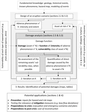
Fig. 1. Idealized scheme of a risk scenario builder tool as obtained after collecting and assimilating high level requirements from a group of
users, geologists and computer scientists.
2 Method: framework for multi-risk scenario builder tools
This section starts with presenting the overall approach. Then, it describes the various steps that are carried out within our proof-of-concept tool.
2.1 Overall approach
Our approach in developing the volcanic risk scenario tool at Mount Cameroon was the following: in a first step, we de-fined high-level requirements for this tool with a group of local users (Ministry of Mines of Cameroon), geologists, ex-perts in scenario builders and computer science, and trans-lated them into low-level requirements for use by develop-ers (Quinet, 2011). This led to defining fundamental require-ments for volcanic risk scenario tools (Fig. 1), which should include the possibility to:
– perform loss computation within a single architecture, allowing automated probabilistic runs;
– integrate spatial features of both adverse events and as-sets (usually GIS-based) in a seamless way;
– jointly compute the damage on both residential build-ings and critical infrastructures; and
– manage scenarios including a succession of different volcanic and geologic phenomena, e.g. through the re-moval of previously destroyed assets.
This last addition was considered most important in order to quantify the consequences of additional adverse events in an already degraded environment.
In a second step, we adapted the seismic risk scenario methodology of Franchin et al. (2011) and Cavalieri et al. (2012) to the context of volcanic risk. The initial toolbox en-ables us to perform an analysis of the physical damages for
2412 P. Gehl et al.: Potential and limitations of risk scenario tools
a wide range of elements at risk (e.g. built areas, network in-frastructures), with a particular focus on critical systems and infrastructures (e.g. major roads, electricity and water net-works). The idea behind it is to facilitate the understanding of vulnerability of essential human activities over the selected territory (systemic vulnerability), beyond the sole assessment of potential physical damages.
We added several modules to the toolbox, including the possibility to (1) merge the damages due to different volcanic phenomena (i.e. “multi-event” scenarios), (2) include various forms of vulnerability models (from deterministic damage matrices to probabilistic fragility curves), and (3) estimate potential damages to cultivated areas and crops, which are an important factor in the case of volcanic risk.
2.2 Representation of adverse events
Since a scenario-based approach has been chosen, probabilis-tic hazard assessment is considered out of the scope of this study and deterministic maps displaying the intensity and ex-tent of hypothesised adverse events are therefore considered as inputs. These have been previously computed or evaluated through various techniques (e.g. event trees, computed haz-ard models, expert elicitation and so forth).
The various adverse events resulting from a volcanic erup-tion are characterised by a damage mechanism and an in-tensity measure, which can be specific to the type of ele-ments they affect. For instance, tephra fall is one type of ad-verse event; for buildings, the damaging mechanism is ver-tical static load (i.e. intensity measure is load in kPa), while it is simply burial (i.e. intensity measure is thickness in cm) with respect to roads or airport runways. This type of hazard decomposition has been discussed by Thierry et al. (2007) and it is carried out here for the following adverse events: tephra fall, lava flows, lahars, debris flows, pyroclastic den-sity currents, blast effects, ballistic blocks, flank collapses, and, although not necessarily related to an eruption, land-slides and earthquakes.
In practice, once a given scenario has been designed, ad-verse events are drawn in a geographical information system (GIS) and the time series of intensity maps are directly im-ported into the toolbox. This modelling choice implies some intensity level bins to define the polygons (see Appendix A). Neri et al. (2013) provide an approach on how to define these bins.
2.3 Inventory of exposed elements
Any risk analysis starts with an inventory of exposed peo-ple, or elements of the built and natural environment over the selected territory. These assets can be classified into three categories:
– Built and cultivated areas: they represent crop fields or industrial plantations, as well as residential build-ings. These data are represented as polygons, whose at-tributes can be typology percentages, number of build-ings, population density (for built areas) or crop type (for cultivated areas).
– Networks: they include all types of lifeline networks (e.g. electric power, water or gas supply) as well as transportation networks (e.g. roads or railways). Each network is represented by a set of polylines and points. – Critical facilities: these point-like components rep-resent strategic buildings such as health-care build-ings, decision centres or law enforcement departments. These important structures are treated as single ob-jects, as opposed to regular residential buildings, and their attributes include information about their relative importance before, during and after the crisis.
Similarly to the hazard input, a GIS-format map for each type of exposed element is imported into the toolbox envi-ronment. In the case of built or cultivated areas, data are pro-jected on a mesh grid composed of a series of cells; a refine-ment algorithm has been developed by Cavalieri et al. (2012) in order to generate variable-sized cells, smaller cells being concentrated around the borders of the polygons. The pro-jection of attributes such as population density or building ty-pologies into each cell is carried out by pondering the respec-tive area of each census polygon within the cell; this means that the attributes are represented and averaged as a propor-tion of the overall cell size. Polylines are also discretized into a series of straight segments, so that they can be defined by only the coordinates of the two extremities; as will be shown in the next subsection, the length of the segment is of little importance and therefore there is no need to carry out further discretization. Finally, point-like objects are imported as they are.
In parallel to this data projection, a taxonomy of the con-sidered assets is proposed in order to classify them in a set of organised systems, following an object-oriented structure. This architecture is slightly adapted from the one introduced by Cavalieri et al. (2012) and it is represented in Fig. 2 as a class diagram in UML notation (Unified Modeling Lan-guage). This formalization allows us to define classes for objects with similar features and the inheritance property of object-oriented programming also gives the possibility to pass along the same attributes to subclasses belonging to the same superclass. This approach can prove very useful to or-ganise the asset inventory in the eventuality of a functionality analysis, since all sets of exposed elements can be grouped into the respective system they are composing. In Fig. 2, the water network has been expanded in order to show the differ-ent layers in the invdiffer-entory description, from compondiffer-ent level to system level. Finally, depending on the role they play in
P. Gehl et al.: Potential and limitations of risk scenario tools 2413
4 Gehl et al.: Potential and limitations of risk scenario tools in volcanic areas through an example in Mount Cameroon categories:
– built and cultivated areas: they represent crops fields or industrial plantations, as well as residential build-ings. These data are represented as polygons, whose
at-240
tributes can be typology percentages, number of build-ings, population density (for built areas) or crop type (for cultivated areas).
– networks: they include all types of lifeline networks (e.g. electric power, water or gas supply) as well as
245
transportation networks (e.g. roads or railways). Each network is represented by a set of polylines and points. – critical facilities: these point-like components represent
strategic buildings such as health-care buildings, deci-sion centers or law enforcement departments. These
250
important structures are treated as single objects, as op-posed to regular residential buildings and their attributes include information about their relative importance be-fore, during and after the crisis.
Similarly to the hazard input, a GIS-format map for each
255
type of exposed elements is imported into the toolbox en-vironment. In the case of built or cultivated areas, data are projected on a mesh grid composed of a series of cells: a refinement algorithm has been developed by Cavalieri et al. (2012) in order to generate variable-sized cells, smaller cells
260
being concentrated around the borders of the polygons. The projection of attributes such as population density or build-ing typologies into each cell is carried out by ponderbuild-ing the respective area of each census polygon within the cell: this means that the attributes are represented and averaged as a
265
proportion of the overall cell size. Polylines are also dis-cretized into a series of straight segments, so that they can be defined by only the coordinates of the two extremities: as will be shown in the next sub-section, the length of the seg-ment is of little importance and therefore there is no need to
270
carry out further discretization. Finally, point-like objects are imported as they are.
In parallel to this data projection, a taxonomy of the con-sidered assets is proposed in order to classify them in a set of organised systems, following an object-oriented structure.
275
This architecture is slightly adapted from the one introduced by Cavalieri et al. (2012) and it is represented in Figure 2, as a class diagram in UML notation (Unified Modelling Lan-guage). This formalization allows to define classes for ob-jects with similar features and the inheritance property of
280
object-oriented programming also gives the possibility to pass along the same attributes to sub-classes belonging to the same superclass. This approach can prove very useful to organize the asset inventory in the eventuality of a func-tionality analysis, since all sets of exposed elements can be
285
grouped into the respective system they are composing. In Figure 2, the water network has been expanded in order to show the different layers in the inventory description, from
Fig. 2. UML (Unified Modeling Language) class diagram of the
studied infrastructure, adapted from Cavalieri et al. (2012)
component-level to system-level. Finally, depending on the role they play in the system, components of a network can be
290
assigned different characteristics (e.g. linear objects become pipelines, points objects can either be source, distribution or storage nodes), which can be used to perform a network anal-ysis subsequently to the physical damage analanal-ysis.
The way this object-oriented architecture is used to model
295
infrastructures is illustrated in Figure 3, using the example of the water supply system. The attributes of the infrastructure components that are described in the GIS dataset are used to assign them to different classes and to characterize them with properties such as geographic location, material type,
capac-300
ity, network connectivity or vulnerability model. Another advantage of the object-oriented approach lies in its flexibil-ity, as it always allows to add modules for extra components and systems, depending on the specific needs of each given case-study.
305
2.4 Projection of adverse event intensities on vulnerable sites
The next step consists of the superposition of both adverse events and exposed elements layers, resulting in the estima-tion of the intensity level at each vulnerable site for each
vol-310
canic phenomenon. This procedure depends on the type of object that is considered:
– For point-like elements, it is very straightforward since
Fig. 2. UML (Unified Modeling Language) class diagram of the
studied infrastructure, adapted from Cavalieri et al. (2012).
the system, components of a network can be assigned dif-ferent characteristics (e.g. linear objects become pipelines; point objects can either be source, distribution or storage nodes), which can be used to perform a network analysis sub-sequently to the physical damage analysis.
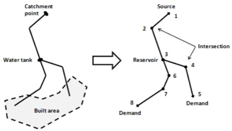
The way this object-oriented architecture is used to model infrastructures is illustrated in Fig. 3, using the example of the water supply system. The attributes of the infrastructure components that are described in the GIS dataset are used to assign them to different classes and to characterise them with properties such as geographic location, material type, capac-ity, network connectivity or vulnerability model. Another ad-vantage of the object-oriented approach lies in its flexibility, as it always allows us to add modules for extra components and systems, depending on the specific needs of each given case study.
2.4 Projection of adverse event intensities on vulnerable sites
The next step consists of the superposition of both adverse event and exposed element layers, resulting in the estimation of the intensity level at each vulnerable site for each volcanic phenomenon. This procedure depends on the type of object that is considered:
– For point-like elements, it is very straightforward since the intensity level is the same as the one of the adverse event polygon where the point is located.
Gehl et al.: Potential and limitations of risk scenario tools in volcanic areas through an example in Mount Cameroon 5
Fig. 3. Modelling example of the part of a water supply system,
using the object-oriented structure
the intensity level is the same as the one of the adverse event polygon where the point is located.
315
– For linear elements, the intensity polygons correspond-ing to each adverse event (see Neri et al., 2013, in this issue) are projected along the length of the exposed seg-ment, which is then assigned different percentages of different intensity levels (see top of Figure 4). This
ap-320
proach allows the user to account precisely for the ex-act intensity level on each linear element, whatever its length.
– For projected cells (i.e. built and cultivated areas), the same approach as for the linear elements is used and it is
325
in agreement with one of the options proposed by Kaye (2007). The event’s intensity polygons are intersected with each cell and area percentages of intensity are then assigned to the cell (see top of Figure 4).
Finally, it has to be kept in mind that this procedure
re-330
lies on the input of adverse event intensity maps that are vector-based, i.e. polygons of binned values of intensity lev-els, as opposed to raster maps, which would require other techniques such as interpolation.
2.5 Damage analysis through fragility models
335
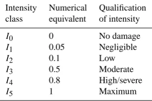
The potential physical damage of exposed elements can only be evaluated once some prerequisite definitions are set, such as a damage scale for each type of component (Blong, 2003), an intensity scale for each type of hazard and, finally, a vul-nerability model that links the input intensity and the
re-340
sulting damage (Thierry et al., 2008). The existing litera-ture on vulnerability to volcanic hazards contains a variety of very disparate models, ranging from simple binary ones (i.e. the asset is destroyed if it is exposed to the volcanic phe-nomenon, whatever its intensity) to gradual damage-intensity
345
matrices (e.g. Wilson et al., 2012, ; where some thresh-old values of tephra loads are proposed for the vulnerability
Fig. 4. (Top) Hazard projection procedure on linear and area-like
vulnerable sites and (Bottom) Example of damage analysis for a hypothetical case, where, by way of example, the edge is assigned a deterministic model, and the cell a probabilistic model for which the cell contains a proportion%T1of building typology 1, with a collapse fragility function.
of utility networks) or even to more elaborate probabilistic fragility functions (i.e. the probability of reaching or exceed-ing the damage state given the intensity level), as shown in
350
the review by Jenkins and Spence (2013).
All types of vulnerability models may be used in the de-veloped toolbox, which assigns one specific vulnerability model to each type of exposed element and each type of phe-nomenon. For deterministic models (i.e. damage-intensity
355
matrices), the event’s intensity levels at each site are trans-lated into other bins of values (i.e. the actual intensities used to evaluate the damage) and then they directly yield the dis-crete damage of the exposed element (see Figure 4). In the case of probabilistic models (i.e. fragility functions), a
sam-360
pling procedure using a standard uniform variable is carried out, in order to check whether the exposed element reaches the damage state or not (see bottom of Figure 4).
When using probabilistic functions, it is necessary to per-form numerous simulation runs to get stable estimates of
365 Fig. 3. Modelling example of the part of a water supply system,
using the object-oriented structure.
– For linear elements, the intensity polygons corre-sponding to each adverse event (see Neri et al., 2013, in this issue) are projected along the length of the ex-posed segment, which is then assigned different per-centages of different intensity levels (see top of Fig. 4). This approach allows the user to account precisely for the exact intensity level on each linear element, what-ever its length.
– For projected cells (i.e. built and cultivated areas), the same approach as for the linear elements is used and it is in agreement with one of the options proposed by Kaye (2007). The event’s intensity polygons are inter-sected with each cell and area percentages of intensity are then assigned to the cell (see top of Fig. 4). Finally, it has to be kept in mind that this procedure re-lies on the input of adverse event intensity maps that are vector-based, i.e. polygons of binned values of intensity lev-els, as opposed to raster maps, which would require other techniques such as interpolation.
2.5 Damage analysis through fragility models
The potential physical damage of exposed elements can only be evaluated once some prerequisite definitions are set, such as a damage scale for each type of component (Blong, 2003), an intensity scale for each type of hazard and, finally, a vul-nerability model that links the input intensity and the re-sulting damage (Thierry et al., 2008). The existing litera-ture on vulnerability to volcanic hazards contains a variety of very disparate models, ranging from simple binary ones (i.e. the asset is destroyed if it is exposed to the volcanic phe-nomenon, whatever its intensity) to gradual damage-intensity matrices (e.g. Wilson et al., 2012, where some threshold values of tephra loads are proposed for the vulnerability of utility networks), or even to more elaborate probabilistic fragility functions (i.e. the probability of reaching or exceed-ing the damage state given the intensity level), as shown in the review by Jenkins et al. (2013).
2414 P. Gehl et al.: Potential and limitations of risk scenario tools
Gehl et al.: Potential and limitations of risk scenario tools in volcanic areas through an example in Mount Cameroon 5
Fig. 3. Modelling example of the part of a water supply system,
using the object-oriented structure
the intensity level is the same as the one of the adverse event polygon where the point is located.
315
– For linear elements, the intensity polygons correspond-ing to each adverse event (see Neri et al., 2013, in this issue) are projected along the length of the exposed seg-ment, which is then assigned different percentages of different intensity levels (see top of Figure 4). This
ap-320
proach allows the user to account precisely for the ex-act intensity level on each linear element, whatever its length.
– For projected cells (i.e. built and cultivated areas), the same approach as for the linear elements is used and it is
325
in agreement with one of the options proposed by Kaye (2007). The event’s intensity polygons are intersected with each cell and area percentages of intensity are then assigned to the cell (see top of Figure 4).
Finally, it has to be kept in mind that this procedure
re-330
lies on the input of adverse event intensity maps that are vector-based, i.e. polygons of binned values of intensity lev-els, as opposed to raster maps, which would require other techniques such as interpolation.
2.5 Damage analysis through fragility models
335
The potential physical damage of exposed elements can only be evaluated once some prerequisite definitions are set, such as a damage scale for each type of component (Blong, 2003), an intensity scale for each type of hazard and, finally, a vul-nerability model that links the input intensity and the
re-340
sulting damage (Thierry et al., 2008). The existing litera-ture on vulnerability to volcanic hazards contains a variety of very disparate models, ranging from simple binary ones (i.e. the asset is destroyed if it is exposed to the volcanic phe-nomenon, whatever its intensity) to gradual damage-intensity
345
matrices (e.g. Wilson et al., 2012, ; where some thresh-old values of tephra loads are proposed for the vulnerability
Fig. 4. (Top) Hazard projection procedure on linear and area-like
vulnerable sites and (Bottom) Example of damage analysis for a hypothetical case, where, by way of example, the edge is assigned a deterministic model, and the cell a probabilistic model for which the cell contains a proportion%T1of building typology 1, with a collapse fragility function.
of utility networks) or even to more elaborate probabilistic fragility functions (i.e. the probability of reaching or exceed-ing the damage state given the intensity level), as shown in
350
the review by Jenkins and Spence (2013).
All types of vulnerability models may be used in the de-veloped toolbox, which assigns one specific vulnerability model to each type of exposed element and each type of phe-nomenon. For deterministic models (i.e. damage-intensity
355
matrices), the event’s intensity levels at each site are trans-lated into other bins of values (i.e. the actual intensities used to evaluate the damage) and then they directly yield the dis-crete damage of the exposed element (see Figure 4). In the case of probabilistic models (i.e. fragility functions), a
sam-360
pling procedure using a standard uniform variable is carried out, in order to check whether the exposed element reaches the damage state or not (see bottom of Figure 4).
When using probabilistic functions, it is necessary to per-form numerous simulation runs to get stable estimates of
365
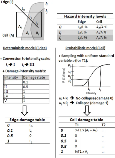
Fig. 4. Top: hazard projection procedure on linear and area-like
vul-nerable sites. Bottom: example of damage analysis for a hypothet-ical case, where, by way of example, the edge is assigned a deter-ministic model, and the cell a probabilistic model for which the cell
contains a proportion %T1 of building typology 1, with a collapse
fragility function.
All types of vulnerability models may be used in the de-veloped toolbox, which assigns one specific vulnerability model to each type of exposed element and each type of phe-nomenon. For deterministic models (i.e. damage-intensity matrices), the event’s intensity levels at each site are trans-lated into other bins of values (i.e. the actual intensities used to evaluate the damage) and then they directly yield the dis-crete damage of the exposed element (see Fig. 4). In the case of probabilistic models (i.e. fragility functions), a sampling procedure using a standard uniform variable is carried out, in order to check whether the exposed element reaches the damage state or not (see bottom of Fig. 4).
When using probabilistic functions, it is necessary to per-form numerous simulation runs to get stable estimates of the loss statistics. Also, since buildings are usually well stud-ied components, they can for instance be assigned fragility functions with respect to tephra fall or pyroclastic density currents; in the proposed approach, the damage analysis of buildings is then performed at the scale of each cell, for each typology present, which means that the sampling procedure
will assign the same damage state to all buildings of the same typology within the same cell.
Finally, the results for each exposed element are presented in a damage table, which indicates the length (or the area or the proportion of buildings or crops) that is assigned to each of the damage states (see Fig. 4). This representation is very useful as an output, as it enables us to quantify the losses in terms of destroyed or impaired assets (e.g. number of km of destroyed power lines or number of collapsed houses). In parallel, for each network, the toolbox also indicates which edges or nodes are considered damaged (i.e. an edge is con-sidered damaged or non-functioning if it contains at least a portion that is in a non-intact damage state), which enables us to update the connectivity of the whole network in order to estimate its functionality loss in a degraded state.
2.6 The case of scenarios composed of a succession of events
While the procedure described above is a straightforward adaptation of previous methods in the field of volcanic risk (EXPLORIS Consortium, 2005; Kaye, 2007) or seismic risk (SYNER-G, 2009–2013), another important issue that has not been fully addressed yet is the analysis of the impact of successive volcanic phenomena within a single eruption sce-nario. When running damage analysis from successive haz-ards, the inventory of exposed assets has to be updated af-ter each single phenomenon simulation, so that the impact of the subsequent phenomenon is accurately estimated (i.e. computation over a degraded set of exposed elements and not the initial intact one). This discussion reveals the need for state-dependent fragility models that should be able to quantify further damage probabilities based on the current state of each element; for instance, buildings with collapsed roofs due to a previous tephra fall may prove much more vul-nerable to other types of hazards. However, the current state of the literature does not yet propose such advanced fragility models for all possible combinations of volcanic hazards and exposed elements, despite some recent efforts (Zuccaro et al., 2008; Zuccaro and De Gregorio, 2013) that have proposed some fragility functions for cumulative damages due to vari-ous phenomena (i.e. earthquakes, dynamic lateral pressures, tephra loads and high temperatures).
Still, an “inventory removal” algorithm was implemented, which accounts for the assets that have already been dam-aged and should not be included in the next damage analysis, at least for the estimation of the lesser damage states they have already reached. This idea has also been raised by Kaye (2007), and we propose here a simple way to apply it. Basi-cally, each object is assigned one damage table for each type of adverse event considered in the scenario (i.e. each phe-nomenon is considered as a unique event), as well as a global damage table that is updated after the simulation of each phenomenon (i.e. a damage table for the whole scenario). The important advantages of using this approach here are
P. Gehl et al.: Potential and limitations of risk scenario tools 2415
6
Gehl et al.: Potential and limitations of risk scenario tools in volcanic areas through an example in Mount Cameroon
the loss statistics.Also, since buildings are usually well
stud-ied components, they can for instance be assigned fragility
functions with respect to tephra fall or pyroclastic density
currents: in the proposed approach, the damage analysis of
buildings is then performed at the scale of each cell, for each
370
typology present, which means that the sampling procedure
will assign the same damage state to all buildings of the same
typology within the same cell.
Finally, the results for each exposed element are presented
in a damage table, which indicates the length (or the area or
375
the proportion of buildings or crops) that is assigned to each
of the damage states (see Figure 4). This representation is
very useful as an output, as it enables to quantify the losses
in terms of destroyed or impaired assets (e.g. number of km
of destroyed power lines or number of collapsed houses). In
380
parallel, for each network, the toolbox also indicates which
edges or nodes are considered damaged (i.e. an edge is
con-sidered damaged or non-functioning if it contains at least a
portion that is in a non-intact damage state), which enables
to update the connectivity of the whole network in order to
385
estimate its functionality loss in a degraded state.
2.6
The case of scenarios composed of a succession of
events
While the procedure described above is a straightforward
adaptation of previous methods in the field of volcanic risk
390
(EXPLORIS Consortium, 2005; Kaye, 2007) or seismic risk
(SYNER-G, 2009–2013), another important issue that has
not been fully addressed yet is the analysis of the impact of
successive volcanic phenomena within a single eruption
sce-nario. When running damage analysis from sucessive
haz-395
ards, the inventory of exposed assets has to be udapted after
each single phenomenon simulation, so that the impact of the
subsequent phenomenon is accurately estimated (i.e.
com-putation over a degraded set of exposed elements and not
the initial intact one). This discussion reveals the need for
400
state-dependent fragility models that should be able to
quan-tify further damage probabilities based on the current state
of each element: for instance, buildings with collapsed roofs
due to a previous tephra fall may prove much more
vulner-able to other types of hazards. However, the current state
405
of the literature does not yet propose such advanced fragility
models for all possible combinations of volcanic hazards and
exposed elements, despite some recent efforts (Zuccaro et al.,
2008; Zuccaro and De Gregorio, 2013) that have proposed
some fragility functions for cumulative damages due to
vari-410
ous phenomena (i.e. earthquakes, dynamic lateral pressures,
tephra loads and high temperatures).
Still, an inventory removal algorithm was implemented,
which accounts for the assets that have already been
dam-aged and should not be included in the next damage
anal-415
ysis, at least for the estimation of the lesser damage states
they have already reached. This idea has also been raised by
Kaye (2007), and we propose here a simple way to apply it.
Fig. 5.
Flowchart implemented in the toolbox for a multi-hazard
scenario
Basically, each object is assigned one damage table for each
type of adverse event considered in the scenario (i.e. each
420
phenomenon is considered as a unique event), as well as a
global damage table that is updated after the simulation of
each phenomenon (i.e. a damage table for the whole
sce-nario). The two important advantages of using this approach
here are twofold: first, the inventory removal algorithm could
425
readily integrate damage-state-dependent fragility functions,
if and when such models are developed in the future;
sec-ondly, for stakeholders such as the civil security, it is
impor-tant for preparedness exercise to evaluate (even roughly) how
damages may occur over the time (e.g. over a few hours or a
430
few weeks): their ability to respond will be different
depend-ing on the temporal dynamic of the damagdepend-ing events. The
different steps of a scenario run are summed up in Figure 5.
The way the global damage table is updated is based on
the following rules:
435
–
For point-like objects, there is only one possible damage
state at once. If a phenomenon induces heavier
dam-age than the previous one, the damdam-age state is updated.
Otherwise, if the induced damage is less than its current
state, the object remains in the same state.
440
–
The same procedure applies for linear or area-like
ob-jects, with keeping in mind however that portions of the
object can be assigned to different damage states at the
same time. This leads to less trivial updating equations,
since all damage states of the object have to be udapted,
445
based on the area or length affected by the next
damag-ing phenomenon (see Figure 6).
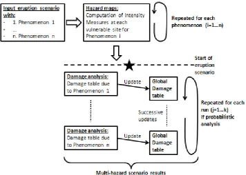
Fig. 5. Flow chart implemented in the toolbox for a multi-hazard scenario.
twofold. First, the inventory removal algorithm could read-ily integrate damage-state-dependent fragility functions, if and when such models are developed in the future. Secondly, for stakeholders such as the civil security, it is important for preparedness exercises to evaluate (even roughly) how dam-ages may occur over the time (e.g. over a few hours or a few weeks); their ability to respond will be different depending on the temporal dynamic of the damaging events. The differ-ent steps of a scenario run are summed up in Fig. 5.
The way the global damage table is updated is based on the following rules:
– For point-like objects, there is only one possible dam-age state at once. If a phenomenon induces heavier damage than the previous one, the damage state is up-dated. Otherwise, if the induced damage is less than its current state, the object remains in the same state. – The same procedure applies for linear or area-like
ob-jects, with keeping in mind however that portions of the object can be assigned to different damage states at the same time. This leads to less trivial updating equa-tions, since all damage states of the object have to be updated, based on the area or length affected by the next damaging phenomenon (see Fig. 6).
Gehl et al.: Potential and limitations of risk scenario tools in volcanic areas through an example in Mount Cameroon 7
Fig. 6. Update procedure for a cell object (the same applies for
edges), containing the building typology 1 over an areaT1.aiand birepresent the areas of impacted buildings.Diis the damage state, according to an hypothetical damage scale.
3 Application to a case-study in the Mount Cameroon area
This approach is then applied to hypothesised scenarios
450
around Mount Cameroon, an active volcano located in the South-West part of Cameroon, in the Fako district.
3.1 Data inventory
This case-study benefits from a previous study on Mount Cameroon, conducted by Thierry et al. (2008) in the frame
455
of the GRINP project (Thierry et al., 2006). Extensive in-ventory field work, as well as the use of GIS databases made available by the Ministry of Industry, Mines and Technologi-cal Development of Cameroon (MINIMIDT), have led to the identification of the following systems, which are considered
460
in the scenario implementation (see Appendix B):
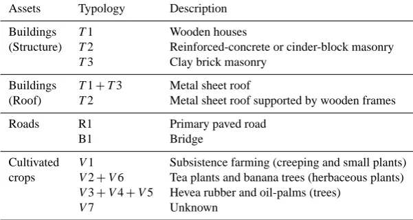
– Built areas: three main structural typologies have been identified (i.e.62.8%of T1: wooden houses with metal sheet roofs; 33.1%of T2: reinforced-concrete or cin-derblock masonry buildings with metal sheet roofs
sup-465
ported by wooden frames;4.1%of T3: clay brick ma-sonry buildings with metal sheet roofs), but no data are available on the specific proportions of these typologies within each built area polygon. This information only exists at the global level and therefore the same
propor-470
tions are applied to all built areas, as a very rough
9.0° E 9.2° E 9.4° E 9.6° E 4.0° N
4.2° N 4.4° N 4.6° N
Cameroon Line Fako District Built areas Population per km²
0 − 45 46 − 126 127 − 355 355 − 6747
Fig. 7. Projection of built areas around Mount Cameroon on the
generated mesh grid and representation of population density within cells
proximation. Moreover, no information on the number of buildings has been gathered and therefore the build-ings (and the associated losses) are merely represented as percentages of the total built area. Finally, a dataset
475
with the population amount within each built area poly-gon is available, allowing to compute specific popula-tion densities (see Figure 7).
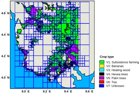
– Cultivated areas with crop types: they are represented as crop polygons, each one being assigned a specific type
480
(i.e. subsistence farming or industrial plantations pro-ducing bananas, heating wood, hevea trees, palm trees or tea). The repartition of different crop types around Mount Cameroon is represented on Figure 8.
– Water supply system: pipelines, water catchments and
485
storage tanks are represented in a GIS database. De-mand nodes are also assigned to the end of each network branch that feeds a built area.
– Electric power network: medium-voltage power lines and electric substations are modelled.
490
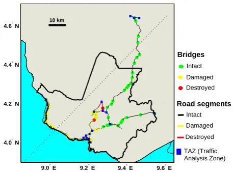
– Road network: only the primary paved road segments are considered, as well as bridges. Some traffic anal-ysis zones (TAZ) are assigned to some nodes that are located in built areas, thus leaving the opportunity to estimate accessibility loss through the computation of
495
origin-destination paths (Franchin et al., 2011). – Critical facilities: the locations of strategic buildings are
identified and three types are considered (i.e. heath-care centers, decision centers, and law enforcement build-ings).
500 Fig. 6. Update procedure for a cell object (the same applies for
edges), containing the building typology 1 over an areaT1.ai and
birepresent the areas of impacted buildings.Diis the damage state,
according to a hypothetical damage scale.
2416 P. Gehl et al.: Potential and limitations of risk scenario tools
Gehl et al.: Potential and limitations of risk scenario tools in volcanic areas through an example in Mount Cameroon
7
Fig. 6.
Update procedure for a cell object (the same applies for
edges), containing the building typology 1 over an area
T
1
.
a
iand
b
irepresent the areas of impacted buildings.
D
iis the damage state,
according to an hypothetical damage scale.
3
Application to a case-study in the Mount Cameroon
area
This approach is then applied to hypothesised scenarios
450
around Mount Cameroon, an active volcano located in the
South-West part of Cameroon, in the Fako district.
3.1
Data inventory
This case-study benefits from a previous study on Mount
Cameroon, conducted by Thierry et al. (2008) in the frame
455
of the GRINP project (Thierry et al., 2006). Extensive
in-ventory field work, as well as the use of GIS databases made
available by the Ministry of Industry, Mines and
Technologi-cal Development of Cameroon (MINIMIDT), have led to the
identification of the following systems, which are considered
460
in the scenario implementation (see Appendix B):
–
Built areas: three main structural typologies have been
identified (i.e.
62
.
8%
of T1: wooden houses with metal
sheet roofs;
33
.
1%
of T2: reinforced-concrete or
cin-derblock masonry buildings with metal sheet roofs
sup-465
ported by wooden frames;
4
.
1%
of T3: clay brick
ma-sonry buildings with metal sheet roofs), but no data are
available on the specific proportions of these typologies
within each built area polygon. This information only
exists at the global level and therefore the same
propor-470
tions are applied to all built areas, as a very rough
9.0° E 9.2° E 9.4° E 9.6° E 4.0° N
4.2° N 4.4° N 4.6° N
Cameroon Line
Fako District
Built areas
Population per km²
0 − 45
46 − 126
127 − 355
355 − 6747
Fig. 7.
Projection of built areas around Mount Cameroon on the
generated mesh grid and representation of population density within
cells
proximation. Moreover, no information on the number
of buildings has been gathered and therefore the
build-ings (and the associated losses) are merely represented
as percentages of the total built area. Finally, a dataset
475
with the population amount within each built area
poly-gon is available, allowing to compute specific
popula-tion densities (see Figure 7).
–
Cultivated areas with crop types: they are represented as
crop polygons, each one being assigned a specific type
480
(i.e. subsistence farming or industrial plantations
pro-ducing bananas, heating wood, hevea trees, palm trees
or tea). The repartition of different crop types around
Mount Cameroon is represented on Figure 8.
–
Water supply system: pipelines, water catchments and
485
storage tanks are represented in a GIS database.
De-mand nodes are also assigned to the end of each network
branch that feeds a built area.
–
Electric power network: medium-voltage power lines
and electric substations are modelled.
490
–
Road network: only the primary paved road segments
are considered, as well as bridges. Some traffic
anal-ysis zones (TAZ) are assigned to some nodes that are
located in built areas, thus leaving the opportunity to
estimate accessibility loss through the computation of
495
origin-destination paths (Franchin et al., 2011).
–
Critical facilities: the locations of strategic buildings are
identified and three types are considered (i.e. heath-care
centers, decision centers, and law enforcement
build-ings).
500
Fig. 7. Projection of built areas around Mount Cameroon on the
generated mesh grid and representation of population density within cells.
3 Application to a case study in the Mount Cameroon area
This approach is then applied to hypothesised scenarios around Mount Cameroon, an active volcano located in the south-west part of Cameroon, in the Fako District.
3.1 Data inventory
This case study benefits from a previous study on Mount Cameroon, conducted by Thierry et al. (2008) in the frame of the GRINP project (Thierry et al., 2006). Extensive in-ventory field work as well as the use of GIS databases made available by the Ministry of Industry, Mines and Technologi-cal Development of Cameroon (MINIMIDT) have led to the identification of the following systems, which are considered in the scenario implementation (see Appendix B):
– Built areas: three main structural typologies have been identified (i.e. 62.8 % of T1: wooden houses with metal sheet roofs; 33.1 % ofT2: reinforced-concrete or cinder-block masonry buildings with metal sheet roofs supported by wooden frames; 4.1 % ofT3: clay brick masonry buildings with metal sheet roofs), but no data are available on the specific proportions of these typologies within each built-area polygon. This infor-mation only exists at the global level and therefore the same proportions are applied to all built areas, as a very rough approximation. Moreover, no information on the number of buildings has been gathered, and therefore the buildings (and the associated losses) are merely represented as percentages of the total built area. Fi-nally, a dataset with the population amount within each built-area polygon is available, allowing us to compute specific population densities (see Fig. 7).
8
Gehl et al.: Potential and limitations of risk scenario tools in volcanic areas through an example in Mount Cameroon
9.0° E 9.2° E 9.4° E 9.6° E 4.0° N
4.2° N 4.4° N 4.6° N
Crop type
V1: Subsistence farming V2: Bananas V3: Heating wood V4: Hevea trees V5: Palm trees V6: Tea V7: Unknown
Fig. 8.
Representation of cultivated areas polygons and projection
on the generated mesh grid
3.2
Selection of scenarios
The study of the volcano’s past has suggested that effusive
eruptions with lava flows are the most common volcanic
events (i.e. cracks opening on the flank or near the summit
of the volcano), even though some lakes located in ancient
505
maar craters represent remnants of the occurrence of a few
phreato-magmatic eruptions (Thierry et al., 2008). In
addi-tion, landslides (not linked with a volcanic eruption)
repre-sent a major threat, particularly to the south of the volcano.
The motivation for selecting these scenarios are the
follow-510
ing: first, although minor eruptions are even more likely,
1922-like events are considered as the most representative
type of major event that authorities should be prepared to.
Second, the phreato-magmatic event have not been
docu-mented in historical records, but geological field
investiga-515
tions have demonstrated that such event may occur and
can-not be neglected as they are highly dangerous. The aim of
this second scenario is therefore to raise awareness on a low
probability/high impact event. Finally, the third scenario is
based on a landslide and is aimed at illustrating the
vulnera-520
bility of the regional electrical network to such local events.
All three scenarios were tested. In the following, we focus
on the first one.
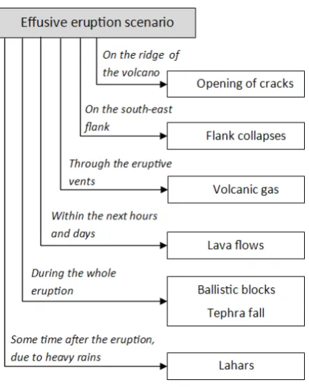
An eruption scenario, based on the sequence of events of
the 1922 eruption, but hypothesised to affect the eastern side,
525
was presented to the authorities in 2008 by Thierry et al.
(2008), using their extensive geological field work, which
in-cludes a study of the volcano summit. It is supposed to start
with the opening of a crack on the volcano edge along the
Cameroon Line, north-west of the Fako district. This crack
530
may induce flank collapses on its south-east side and the
vol-canic gases that are released through the crack generate lava
fountains out of the vent. These lava emissions may
verti-cally eject ballistic blocks and tephra up to a few hundreds of
meters. The tephra can then be dispersed by the wind to the
535
south-west and cover the coast area with a few millimetres of
Fig. 9.
Proposed arbitrary scenario with all associated volcanic
phe-nomena
ash. Finally, once the eruption has slowed down, heavy rains
might fall on the thick tephra layers and other fallouts
accu-mulated on the volcano flanks, thus generating lahars along
the steepest slopes. The sequence of the different volcanic
540
phenomena involved in this hypothetical scenario is
repre-sented in Figure 9.
3.3
Probabilistic impact analysis and results
Now that both adverse event inputs and exposed elements are
clearly identified and formatted, the corresponding
vulnera-545
bility models have to be selected and applied to each
combi-nation of phenomenon - exposed asset. As described above,
the developed toolbox enables to host different vulnerability
models, whether probabilistic or deterministic. Since the
ob-jective of this study is not as much to perform an accurate
550
scenario than to demonstrate the feasibility of our approach,
some vulnerability models have been chosen, even though
they may not be the most adequate or recent ones, and they
are described in Table 1.
Damage matrix models are tables that give intensity ranges
555
(e.g. tephra thickness, see Appendix C) within which the
ex-posed element is assigned a given damage state (e.g. damage
ratio expressed in percentages). Binary models just check
if the exposed element is located within the hazard
occur-rence area, resulting in complete damage if this is the case.
560
Finally, fragility curves used here represent the probability
of roof collapse given a level of tephra load. For the roof
types encountered in this study, a median load of
2 kPa
is
assigned to simple metal sheet roofs (i.e. building typologies
T1 and T3) and a load of
3 kPa
is set for metal sheet roofs
565
with wooden frame support (i.e. building typology T2). The
Fig. 8. Representation of cultivated-area polygons and projection on
the generated mesh grid.
– Cultivated areas with crop types: they are represented as crop polygons, each one being assigned a specific type (i.e. subsistence farming or industrial plantations producing bananas, heating wood, hevea trees, palm trees or tea). The repartition of different crop types around Mount Cameroon is represented in Fig. 8. – Water supply system: pipelines, water catchments and
storage tanks are represented in a GIS database. De-mand nodes are also assigned to the end of each net-work branch that feeds a built area.
– Electric power network: medium-voltage power lines and electric substations are modelled.
– Road network: only the primary paved road segments are considered, as well as bridges. Some traffic anal-ysis zones (TAZ) are assigned to some nodes that are located in built areas, thus leaving the opportunity to estimate accessibility loss through the computation of origin-destination paths (Franchin et al., 2011). – Critical facilities: the locations of strategic buildings
are identified and three types are considered (i.e. heath-care centres, decision centres, and law enforcement buildings).
3.2 Selection of scenarios
The study of the volcano’s past has suggested that effusive eruptions with lava flows are the most common volcanic events (i.e. cracks opening on the flank or near the summit of the volcano), even though some lakes located in ancient maar craters represent remnants of the occurrence of a few phreatomagmatic eruptions (Thierry et al., 2008). In addi-tion, landslides (not linked with a volcanic eruption) repre-sent a major threat, particularly to the south of the volcano.
P. Gehl et al.: Potential and limitations of risk scenario tools 2417
The motivations for selecting these scenarios are the fol-lowing: first, although minor eruptions are even more likely, 1922-like events are considered as the most representative type of major event that authorities should be prepared for. Second, the phreatomagmatic events have not been docu-mented in historical records, but geological field investiga-tions have demonstrated that such events may occur and can-not be neglected as they are highly dangerous. The aim of this second scenario is therefore to raise awareness on low probability/high impact events. Finally, the third scenario is based on a landslide and is aimed at illustrating the vulnera-bility of the regional electrical network to such local events. All three scenarios were tested. In the following, we focus on the first one.
An eruption scenario, based on the sequence of events of the 1922 eruption, but hypothesised to affect the eastern side, was presented to the authorities in 2008 by Thierry et al. (2008), using their extensive geological field work which in-cludes a study of the volcano summit. It is supposed to start with the opening of a crack on the volcano edge along the Cameroon line, north-west of the Fako District. This crack may induce flank collapses on its south-east side, and the vol-canic gases that are released through the crack generate lava fountains out of the vent. These lava emissions may verti-cally eject ballistic blocks and tephra up to a few hundreds of metres. The tephra can then be dispersed by the wind to the south-west and cover the coast area with a few millimetres of ash. Finally, once the eruption has slowed down, heavy rains might fall on the thick tephra layers and other fallouts accu-mulated on the volcano flanks, thus generating lahars along the steepest slopes. The sequence of the different volcanic phenomena involved in this hypothetical scenario is repre-sented in Fig. 9.
3.3 Probabilistic impact analysis and results
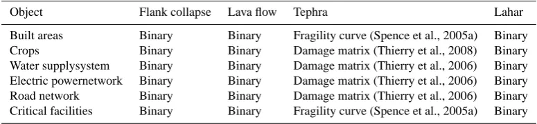
Now that both adverse event inputs and exposed elements are clearly identified and formatted, the corresponding vulnera-bility models have to be selected and applied to each com-bination of phenomenon–exposed asset. As described above, the developed toolbox enables us to host different vulnerabil-ity models, whether probabilistic or deterministic. Since the objective of this study is not so much to perform an accurate scenario as to demonstrate the feasibility of our approach, some vulnerability models have been chosen, even though they may not be the most adequate or recent ones, and they are described in Table 1.
Damage matrix models are tables that give intensity ranges (e.g. tephra thickness, see Appendix C) within which the ex-posed element is assigned a given damage state (e.g. damage ratio expressed in percentages). Binary models just check if the exposed element is located within the hazard occur-rence area, resulting in complete damage if this is the case. Finally, fragility curves used here represent the probability of roof collapse given a level of tephra load. For the roof
8
Gehl et al.: Potential and limitations of risk scenario tools in volcanic areas through an example in Mount Cameroon
9.0° E 9.2° E 9.4° E 9.6° E 4.0° N
4.2° N 4.4° N 4.6° N
Crop type
V1: Subsistence farming V2: Bananas V3: Heating wood V4: Hevea trees V5: Palm trees V6: Tea V7: Unknown
Fig. 8.
Representation of cultivated areas polygons and projection
on the generated mesh grid
3.2
Selection of scenarios
The study of the volcano’s past has suggested that effusive
eruptions with lava flows are the most common volcanic
events (i.e. cracks opening on the flank or near the summit
of the volcano), even though some lakes located in ancient
505
maar craters represent remnants of the occurrence of a few
phreato-magmatic eruptions (Thierry et al., 2008). In
addi-tion, landslides (not linked with a volcanic eruption)
repre-sent a major threat, particularly to the south of the volcano.
The motivation for selecting these scenarios are the
follow-510
ing: first, although minor eruptions are even more likely,
1922-like events are considered as the most representative
type of major event that authorities should be prepared to.
Second, the phreato-magmatic event have not been
docu-mented in historical records, but geological field
investiga-515
tions have demonstrated that such event may occur and
can-not be neglected as they are highly dangerous. The aim of
this second scenario is therefore to raise awareness on a low
probability/high impact event. Finally, the third scenario is
based on a landslide and is aimed at illustrating the
vulnera-520
bility of the regional electrical network to such local events.
All three scenarios were tested. In the following, we focus
on the first one.
An eruption scenario, based on the sequence of events of
the 1922 eruption, but hypothesised to affect the eastern side,
525
was presented to the authorities in 2008 by Thierry et al.
(2008), using their extensive geological field work, which
in-cludes a study of the volcano summit. It is supposed to start
with the opening of a crack on the volcano edge along the
Cameroon Line, north-west of the Fako district. This crack
530
may induce flank collapses on its south-east side and the
vol-canic gases that are released through the crack generate lava
fountains out of the vent. These lava emissions may
verti-cally eject ballistic blocks and tephra up to a few hundreds of
meters. The tephra can then be dispersed by the wind to the
535
south-west and cover the coast area with a few millimetres of
Fig. 9.
Proposed arbitrary scenario with all associated volcanic
phe-nomena
ash. Finally, once the eruption has slowed down, heavy rains
might fall on the thick tephra layers and other fallouts
accu-mulated on the volcano flanks, thus generating lahars along
the steepest slopes. The sequence of the different volcanic
540
phenomena involved in this hypothetical scenario is
repre-sented in Figure 9.
3.3
Probabilistic impact analysis and results
Now that both adverse event inputs and exposed elements are
clearly identified and formatted, the corresponding
vulnera-545
bility models have to be selected and applied to each
combi-nation of phenomenon - exposed asset. As described above,
the developed toolbox enables to host different vulnerability
models, whether probabilistic or deterministic. Since the
ob-jective of this study is not as much to perform an accurate
550
scenario than to demonstrate the feasibility of our approach,
some vulnerability models have been chosen, even though
they may not be the most adequate or recent ones, and they
are described in Table 1.
Damage matrix models are tables that give intensity ranges
555
(e.g. tephra thickness, see Appendix C) within which the
ex-posed element is assigned a given damage state (e.g. damage
ratio expressed in percentages). Binary models just check
if the exposed element is located within the hazard
occur-rence area, resulting in complete damage if this is the case.
560
Finally, fragility curves used here represent the probability
of roof collapse given a level of tephra load. For the roof
types encountered in this study, a median load of
2 kPa
is
assigned to simple metal sheet roofs (i.e. building typologies
T1 and T3) and a load of
3 kPa
is set for metal sheet roofs
565
with wooden frame support (i.e. building typology T2). The
Fig. 9. Proposed arbitrary scenario with all associated volcanic
phenomena.
types encountered in this study, a median load of 2 kPa is as-signed to simple metal sheet roofs (i.e. building typologies
T1 andT3) and a load of 3 kPa is set for metal sheet roofs with wooden frame support (i.e. building typologyT2). The standard deviation of the fragility curves is assumed to be 0.3 (Jenkins and Spence, 2009). Since the fragility model from Spence et al. (2005a) uses tephra load as the intensity mea-sure and since our hazard intensity map is expressed in tephra thickness, a rough conversion is performed by considering a tephra deposit density of 1600 kg m−3(Thierry et al., 2006). This corresponds to the density of wet tephra, which consti-tutes a reasonable assumption, given the rainy climate of the studied region.
As can be seen in Table 1, the scenario relies on a com-bination of both probabilistic and deterministic models, thus requiring us to run multiple analyses of the same scenario to obtain stable statistics of the distribution of the propor-tion of collapsed roofs due to tephra load. Other determinis-tic models yield the same result for each run, however they should be computed simultaneously with the probabilistic ones, since the loss estimation of infrastructures other than buildings is of crucial importance in the eventuality of a sys-temic analysis. The final results of this multi-event scenario can now be aggregated for each system (see Table 2). De-pending on the asset type, losses can be expressed in terms of discrete amounts (e.g. number of destroyed bridges), lengths