Spectral Fatigue Analysis Techniques
Zhihua Hu
A D issertation subm itted for the Degree of
D octor of Philosophy
Departm ent of Mechanical Engineering
University College London
ProQuest Number: 10046186
All rights reserved
INFORMATION TO ALL USERS
The quality of this reproduction is dependent upon the quality of the copy submitted.
In the unlikely event that the author did not send a complete manuscript and there are missing pages, these will be noted. Also, if material had to be removed,
a note will indicate the deletion.
uest.
ProQuest 10046186
Published by ProQuest LLC(2016). Copyright of the Dissertation is held by the Author.
All rights reserved.
This work is protected against unauthorized copying under Title 17, United States Code. Microform Edition © ProQuest LLC.
ProQuest LLC
789 East Eisenhower Parkway P.O. Box 1346
A b stra ct
This thesis presents a practical design tool for wind turbine blades which was de veloped from existing theory on spectral fatigue analysis previously used for off shore platform design. The usual aim with spectral fatigue analysis techniques is to estim ate fatigue damage or some related function such as rainflow ranges from spectral statistics. Monitored structural responses from different wind turbines were used to assess these existing techniques. The best two methods (suitable only for Gaussian stationary and random responses) were found to be Dirlik’s empirical formula and Bishop’s theoretical solution. Various param eters involved in the com putation such as cutoff frequency and clipping ratio were examined. Guidelines for selection of these param eters are also given.
A m ethod based on Bishop’s theoretical solution is extended to include the influence of mean stress. The joint PD F of rainflow cycle and mean stress can be obtained from the response PSD using this method. Because the global mean level information is usually not provided by the PSD, only the relative mean of each rainflow cycle is calculated using this method. The global mean level can then be provided by the designer during the structural analysis stage. This new m ethod was used to analyse the mean stress influence for wind turbine blades using the two monitored structural response histories mentioned above.
A num ber of possible approaches for the spectral fatigue analysis of non- Gaussian response histories are discussed. A m ethod based on Bishop’s theo retical solution is extended to calculate the PD F of rainflow ranges from non- Gaussian response histories specified as a peak trough transition m atrix. Al though this is only a partial solution to the overall problem it still represents a significant breakthrough. It may, for instance, be of use for estim ating rain flow ranges from standardised load sequences specified as turning point matrices. Restricted by the complexity of non-Gaussian processes, especially the lim ited in formation provided by PSD ’s, a universal solution for the transition m atrix and the peak number of the process in unit tim e is currently not available.
T able o f C o n ten ts
A b stra ct ix
Table o f C on ten ts ix
L ist o f F igu res ix
L ist o f Tables ix
L ist o f S ym b ols and A b b rev ia tio n s x
A ck n ow led gem en ts xiii
D ecla ra tio n x iv
1 In tro d u ctio n 1
2 T h eo re tica l background for sp ectra l fa tig u e an alysis 7
2.1 In tro d u c tio n . . . 7
2.2 Fatigue damage a c c u m u la tio n ... 8
2.3 Stress (Strain) cycle c o u n t i n g ... 11
2.4 Stochastic p ro cess... 16
2.4.1 General a s s u m p tio n s ... 16
2.4.2 Probability and m om ents... 16
2.4.3 Correlation f u n c t i o n ... 17
2.4.4 Fourier analysis and s p e c tr u m ... 18
2.4.5 Fast Fourier T ran sfo rm ... 19
2.4.6 Statistics in the frequency d o m a in ... 21
2.5 Spectral analysis and structural dynamics ... 22
2.6 Some useful results from the P S D ... 25
2.6.1 Zero c ro ssin g s... 25
2.6.2 Distribution of E x t r e m a ... 27
2.7 D iscu ssio n ... 29
3 P resen t m eth o d s in use 31 3.1 General background... 31
3.2 Narrow band so lu tio n ... 31
3.3 Correction factor m e t h o d s ... 32
3.3.1 Wirsching’s correct f a c t o r ... 32
3,3.3 Hancock’s equations ... 33
3.4 Tunna’s fo rm u la ... 34
3.5 Dirlik’s f o r m u la ... 34
3.6 Bishop’s theoretical s o lu tio n ... 35
3.7 Madsen fo rm u la ... 36
3.8 D isc u ssio n ... 39
F atigu e A n a ly sis o f W E G M S-1 and H ow den d ata 40 4.1 In tro d u c tio n ... 40
4.2 Analysis p r o g r a m ... 40
4.3 Analysis of WEG MS-1 d a t a ... 43
4.3.1 The WEG MS-1 d a t a ... 43
4.3.2 S — N c u rv e ... 43
4.3.3 Statistical a n a l y s i s ... 44
4.3.4 Fatigue a n a ly s is ... 48
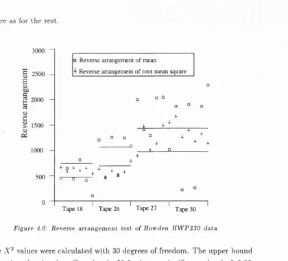
4.4 Analysis of Howden HWP330 d a t a ... 51
4.4.1 HOWDEN HWP330 d a t a ... 51
4.4.2 S — N c u rv e ... 51
4.4.3 Statistical a n a l y s i s ... 51
4.4.4 Fatigue a n a ly s is ... 52
4.5 D isc u ssio n ... 56
C o m p u ta tio n a l con sid eration s in random fatigu e an alysis 58 5.1 Effect of cutoff freq u en cy ... 58
5.2 Length re q u ire m e n t... 63
5.3 Effect of S — N curve slope ... 69
5.4 Selection of clipping ratio ... 73
5.5 Effect of determ inistic components ... 73
5.6 D isc u ssio n ... 76
Influence o f M ean Stress 77 6.1 In tro d u c tio n ... 77
6.2 Goodman relationship ... 78
6.3 Theoretical solution for Gaussian s i g n a l s ... 81
6.3.1 Markov P r o c e s s ... 81
6.3.2 BcLsic formulation of the theoretical s o l u t i o n ... 81
6.3.3 Markov model for rainflow c y c le ... 82
6.3.4 Initial transition and Kowalewski formula ... 84
6.3.5 Long run p r o b a b ility ... 88
6.4 Modification for considering the mean s t r e s s ... 89
6.5 Analysis of WEG data including mean s t r e s s ... 90
6.6 Analysis of Howden data including mean stress ... 93
7 F atigu e analysis for N on -G aussian resp on se h isto ries 97
7.1 In tro d u c tio n ... 97
7.2 M athematical description of non-Gaussian v a ria b le s ... 98
7.2.1 Characteristic functions ... 98
7.2.2 Gram-Charlier E x p a n s io n ... 99
7.2.3 Maximum Entropy M e th o d (M E M )...100
7.3 Statistical description of non-Gaussian p ro c e sse s... 100
7.3.1 Time d o m a i n ...100
7.3.2 Frequency domain ...101
7.4 Present methods for non-Gaussian signal fatigue a n a ly s is ...102
7.4.1 Transformation method ... 102
7.4.2 Weakly non-Gaussian a p p ro x im a tio n ... 102
7.5 Theoretical solution for non-Gaussian stress history analysis . . . 103
7.5.1 Statistic a s p e c t ... 103
7.5.2 Theoretical solution for non-Gaussian r e s p o n s e s ...103
7.6 Peak-trough series r e g e n e ra tio n ...106
7.6.1 Transition m a t r i x ... 106
7.6.2 Load sequence generation ...108
7.7 D isc u ssio n ...109
8 F atigu e analysis for random stress h isto ries w ith d eterm in istic co m p o n en ts 111 8.1 B a c k g ro u n d ... I l l 8.2 Simulation of a stress history with determ inistic components . . . 114
8.2.1 Simulation of a stationary Gaussian p r o c e s s ... 114
8.2.2 Simulation of a stress history with a determ inistic component 116 8.3 Modelling the rainflow range probability d e n s ity ... 124
8.3.1 Gaussian tim e history ...124
8.3.2 Random tim e history with a determ inistic component . . . 125
8.4 Param eter e v a lu a tio n ... 126
8.4.1 Least square te c h n iq u e ... 126
8.4.2 Param eter evaluation for rainflow cycle m o d e ls... 128
8.5 An introduction to neural c o m p u ta tio n ...143
8.5.1 Basic structure of neural n e t w o r k ...143
8.5.2 Mapping N e tw o r k s ...147
8.6 The use of neural networks for fatigue a n a ly s is ... 150
8.6.1 Toolbox for fatigue analysis of random stress histories with deterministic c o m p o n e n t...150
8.6.2 Toolbox of fatigue design for Gaussian stress histories . . . 151
8.7 D iscu ssio n ...154
9 A ssessm en t of th e neural netw ork to o lb o x 165 9.1 In tro d u c tio n ... 165
9.2 Extraction of deterministic c o m p o n en ts... 166
9.2.1 Band pass f i l t e r ... 166
9.2.3 Some comments about the azim uth averaging m ethod . . . 168
9.3 Separation of the Howden d a t a ...168
9.4 Reanalysis of Howden d a t a ... 170
9.5 Result for simulated signals ... 174
9.6 C o n c lu sio n s... 176
10 C on clu sion s and S u g g ested Future W ork 177 10.1 C o n c lu s io n s ... 177
10.2 Suggested future w o r k ...179
R eferen ces 180
A S p ectra l fatigu e an alysis program for G aussian resp o n ses 189
L ist o f F igu res
2.1 A typical 5 - c u r v e ... 8
2.2 The stress-strain hysteresis cy cle... 9
2.3 Rychlik’s definition for rainflow c y c l e ... 13
2.4 Modified definition for rainflow c y c l e ... 13
2.5 'B ishop’s definition for rainflow cycle ... 14
2.6 An example of rainflow cycle counting ... 15
2.7 PSD moments c a l c u l a t i o n ... 21
2.8 A typical sample function of X{ t) and its associated sample functions 26 4.1 Spectrum of n h d a t a... 42
4.2 Rainflow cycle distribution of n b d a t a... 42
4.3 Reverse arrangement test of WEG MS-1 d a t a ... 45
4.4 of WEG MS-1 data for degree 3 0 ... 46
4.5 Rainflow cycle probability density and damage distribution for WEG MS-1 d ata y l2a ... 49
4.6 Reverse arrangement test of Howden HWP330 d a t a ... 52
4.7 Rainflow cycle probability density of Howden d a t a ... 55
4.8 Block effect of Howden data tape 26 3m flapw ise... 57
5.1 Influence of cutoff frequency of WEG MS-1 d ata y 2 7 a ... 60
5.2 Influence of cutoff frequency of Howden data, tape 26 61 5.3 Kowalewski matrices with different cutoff fre q u e n c y ... 62
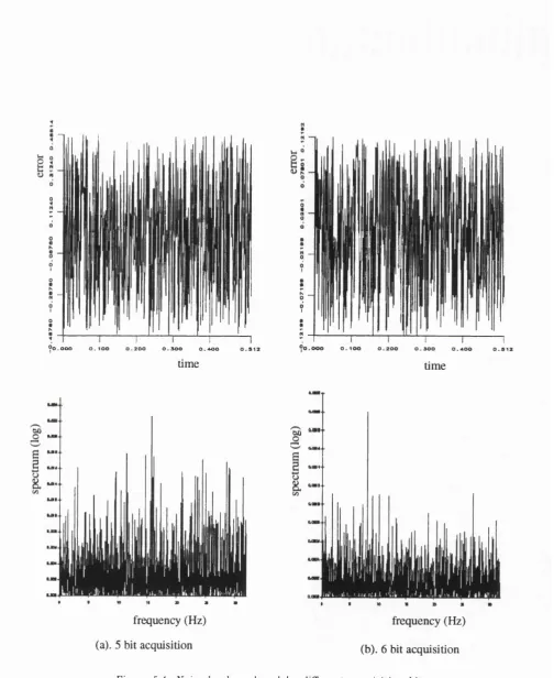
5.4 Noise level produced by different acquisition b it... 64
5.5 Length effect of idealised d a t a ... 65
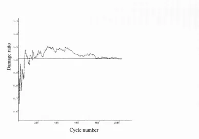
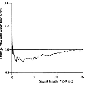
5.6 Length effect of WEG MS-1 data y l 2a ... 65
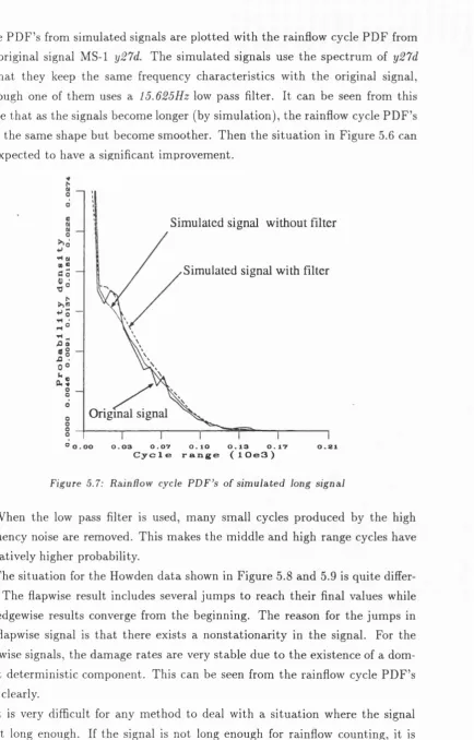
5.7 Rainflow cycle P D F ’s of simulated long s i g n a l ... 66
5.8 Length effect for Howden data tape 27 flapwise s ig n a l... 67
5.9 Length effect for Howden data tape 27 edgewise signal ... 67
5.10 Window size effect: WEG MS-1 data y 2 7 a ... 68
5.11 Effect of S-N curve slope: WEG MS-1 data y 2 7 a ... 70
5.12 Effect of S-N curve slope: WEG MS-1 data y 2 7 d ... 71
5.13 Effect of S-N curve slope: Howden data tape 26 3m flapwise . . . 72
5.14 Effect of S-N curve slope: Howden data tape 26 3m edgewise . . . 72
5.15 Clipping of normal d i s t r i b u t i o n ... 74
5.16 Choice of clipping ratio: WEG data y 2 7 d ... 74
5.17 Choice of clipping ratio: Howden d ata tape 26 3m flapwise . . . . 75
5.18 Choice of clipping ratio: Howden data tape 26 3m edgewise . . . . 75
6.2 S-N curves with different mean ... 79
6.3 Fatigue life - cycle range - mean stress c u r v e ... 79
6.4 Goodman r e l a tio n s h ip ... 80
6.5 Illustration of events Fi, F2, I 3 ... 83
6.6 Markov model for rainflow c y c le ... 84
6.7 Illustration of Kowalewski’s expression... 85
6.8 (a) The trough given peak part of Kowalewski’s expression for a 16 by 16 m atrix.(b) The peak given trough part of Kowalewski^s expression for a 16 by 16 m atrix... 86
6.9 Example of one step transition m atrix.(a) peak to trough, (b) trough to peak ... 86
6.10 Transition m atrix and its equilibrium d is tr ib u tio n ... 87
6.11 The assumption of normality and s t a t i o n a r i t y ... 89
6.12 Example illustrating the method of evaluating p r r{3) for a 16 level p ro c e ss ... 90
6.13 The joint PD F of rainflow range and mean from y 2 7 a ... 92
6.14 The joint PD F of rainflow range and mean from Howden d ata tape 26 3m flapw ise... 95
6.15 The joint PD F of rainflow range and mean from Howden data tape 26 3m e d g e w is e ... 96
7.1 Non-Gaussian transition probability m a trix ... 104
7.2 Rainflow cycle P D F ’s from non-Gaussian transition m atrix . . . . 105
7.3 FALSTAFF m a t r i c e s ... 107
7.4 Load sequence regeneration ...108
7.5 P D F ’s from regenerated load s e q u e n c e ... 109
8.1 The effect of deterministic component in stress history ...112
8.2 The methodology used to develop a combined signal toolbox for fatigue a n a l y s is ... 113
8.3 Harmonic component from s p e c t r u m ...115
8.4 Shapes of spectra u s e d ...119
8.5 Phase check for input sine w aves... 121
8.6 Average of absolute percentage errors of fatigue damage with dif ferent p h a s e 122 8.7 Rainflow cycle probability density function from spectrum 1 . . . 124
8.8 Model for the rainflow cycle probability density f u n c t i o n ... 125
8.9 Curve fitting on weighted and unweighted b a s i s ... 132
8.10 Curve fitting for spectrum no. 1 ... 133
8.11 Least-square fitting results for spectra 6 0 ...136
8.12 A typical neural network a rc h ite c tu re ...145
8.13 A generic processing e le m e n t...145
8.14 Layout of back propagation n etw o rk ...147
8.15 A typical error surface...150
8.16 Convergence path of /i, a , C2 and E [ P ]... 152
8.17 Neural network prediction for spectra 6 0 ... 153
8.19 The rainflow cycle P D F ’s and fatigue damage density functions
from tim e domain analysis and neural network com putation . . . 156
9.1 Azimuth of turbine b la d e ...167
9.2 A sample of azimuth record from HWP330 tape 1 8 ... 169
9.3 The stochastic component of tape 18 3m edgewise s i g n a l ... 171
9.4 Rainflow cycle probability density function from tim e and fre quency domain an aly sis 171 9.5 Howden d ata tape 26 3m edgewise ... 173
9.6 New simulated s ig n a l ...174
9.7 Rainflow cycle P D F ’s from new simulated s ig n a l...175
L ist o f T ables
4.1 MS-1 load ccLses... 43
4.2 Statistical analysis for WEG MS-1 d a t a ... 47
4.3 Fatigue damage rates for WEG MS-1 d a t a ... 50
4.4 Load case of Howden HWP330 d a t a ... 51
4.5 ' Statistical analysis for Howden d a t a ... 53
4.6 Fatigue damage rates for Howden data b=4’0 54 4.7 Fatigue damage rates for Howden data h=8.0 54 4.8 Fatigue damage rates for Howden data b = 1 2 . 0... 56
6.1 Fatigue damage ratio for WEG MS-1 d ata with mean stress . . . 91
6.2 U ltim ate bending moments of Howden d a t a ... 93
6.3 Fatigue damage ratio of Howden data with mean b = 8 . 0... 94
6.4 Fatigue damage ratio of Howden data with mean b = 1 2 . 0... 94
8.1 70 PSD ’s used in stress history simulation ( 1 ) ... 117
8.2 70 PSD ’s used in stress history simulation ( 2 ) ... 118
8.3 Statistical param eters for signals from PSD N o . l ...123
8.4 Model param eters by curve fitting with weight ^^{z) = z (1) . . . 134
8.5 Model param eters by curve fitting with weight (^(z) = z (2) . . . 135
8.6 Fatigue damage rates for fitted model curve with 6 = 5.0 ( 1 ) . . . 137
8.7 Fatigue damage rates for fitted model curve with 6 = 5.0 (2) . . . 138
8.8 Fatigue damage rates for fitted model curve with 6 = 5.0 (3) . . . 139
8.9 Fatigue damage rates for fitted model curve with 6 = 5.0 (4) . . . 140
8.10 Fatigue damage rates for fitted model curve with 6 = 5.0 (5) . . . 141
8.11 Fatigue damage rates for fitted model curve with 6 = 5.0 (6) . . . 142
8.12 Model param eters calculated from neural network toolbox for the 70 PSD ’s use... 157
8.13 Model param eters calculated from neural network toolbox for the 70 PSD ’s use... 158
8.14 Fatigue damage rates from neural toolbox 6 = 5.0 ( 1 ) ... 159
8.15 Fatigue damage rates from neural toolbox 6 = 5.0 ( 2 ) ...160
8.16 Fatigue damage rates from neural toolbox 6 = 5.0 ( 3 ) ...161
8.17 Fatigue damage rates from neural toolbox 6 = 5.0 ( 4 ) ...162
8.18 Fatigue damage rates from neural toolbox 6 = 5.0 ( 5 ) ...163
8.19 Fatigue damage rates from neural toolbox 6 = 5.0 (6) ...164
9.2 Amplitudes of determ inistic components in Howden d ata edgewise s ig n a l s ... 170 9.3 Damage rates of frequency domain results with tim e domain results
for Howden data edgewise signals with b = 5 .0...172 9.4 Damage rates of frequency domain results compared with the time
domain results for the new simulated signals with b = 5 . 0...175 9.5 Damage rates of Dirlik’s formula compared with the tim e domain
L ist o f S ym b o ls and A b b rev ia tio n s
PSD Power Spectral Density Rxx autocorrelation function
PD F Probability Density Function bjiFourier constants DFT Discrete Fourier Transform Wn radius frequency FF T Fast Fourier Transform
%(w)
Fourier integral RAT Reverse Arrangement Test A{u) real part of X {lj)rms root mean square B{u>) imaginary part of X (lû)
5(0-) two sided spectrum
S cycle range G{ f ) one sided spectrum
N cycle number X stochastic process
b inverse slope of S~N curve X first order differential process
k S-N curve intercept X second order differential process
a A K D,n Y Sa ris E[D] E[P] E[0] T P(S) y(t) «+ x(t) P(x) pM X a E{.} (f){u) R.^xy
Chapter 2
crack length
stress (strain) intensity factor m aterial constants
specimen geometry and loading factor cycle stress range
number of cycles with range S
expected fatigue damage expected peak number in unit tim e
expected zero crossing in unit tim e
tim e duration cycle range
probability density function response series
tim e forwards tim e backwards random process
probability distribution of x
probability density function of x
nth order moment
nth order central moment mean value of random process root mean square
m athem atical expectation characteristic function cross-correlation function tim e lag
autocorrelation function
Git ( / ) power spectral density function
Ls A t rrin 7 /m M C K V p (r) T, h(-)
duration of signal
tim e interval width of signal nth order moment of PSD irregularity factor
“m ean” frequency mass m atrix damping m atrix stiffness m atrix deformation loading period of load
unit impulse response function f(zw ) Fourier transform of load p(t) v(t) tim e domain response
y (zw)frequency domain response
H(uj) frequency response function
S(iij) response spectrum u[-] unit step function
number of level crossing number of zero crossing number of extrem a
number of extrem a per unit tim e
Chapter 3
N O
r ( 0)
M()
9+0
R[R^]rr expected damage by rainflow cycle
R[D]n b expected damage
by narrow band solution A(-,-) correction factor
a,c constants
r(-)
Gamma functionSh equivalent stress
er f( ') error function
z normalised cycle range (= S /2y/m^ )
Pr r{z) rainflow cycle range PD F
Cl coefficients in Dirlik’s formula
C2 coefficients in Dirlik’s formula
C3 coefficients in Dirlik’s formula
r factor of
exponential distribution
a factor of Rayleigh distribution
Yi first event in rainflow cycle
Y2 second event in rainflow cycle
Y3 third event in rainflow cycle
probabilities of yi F2O probabilities of Y2
Y3I) probabilities of Y3
ip peak level
kp trough level
dh level interval width
X(t) stochastic signal
Z(t) determ inistic component
Y(t) combined tim e history
X ( t) +Y (t)
Qxi) bandwidth correction term M (-, - , •) confluent hypergeometric
function
Nu num ber of mean upcrossings of deterministic component in one period
Np number of peaks
of determ inistic component in one period
(Tx standard deviation of stochastic process
(Jz standard deviation
of deterministic component
Ck amplitudes of sine waves
4>{t) standard normal distribution
= Slo ^{P)dp = erf{t) ((t) = <j)(t) — f)
'y{t) deterministic component of the combined signal
Chapter 4
N number of signal blocks
A acceptable range for RAT chi-square distribution
X"^ calculated value of chi-square test
K class intervals
fi observed frequency
Fi expected frequency
n number of freedom
a significance level
Xn;a chi-square value with number of degrees n with significance level a
Chapter 5
p clipping ratio
Xmax assumed maxim um value of random process
Chapter 6
& cycle range with mean
SaO cycle range with zero mean Sm mean stress of cycle
Suit ultim ate tensile stress Sy yield stress
/(•!•) conditional probability trough level
0 ( 2 peak level
p .mtn,max0 peak-trough transition probability P transition probability m atrix
Pij element of P
c
absorption stateT transient state
R transition probability from T to
C
Q transition probability within T I transition probability within C,unit m atrix
0 transition probability out of
C,
null m atrix
n
equilibrium distribution of transition probabilityf i long run probability
of transition from
i
to it jHkO Hermite series T coefficient
F(w) Fourier transform of p(x) in exponential distribution
H , entropy of PDF Ot coefficient
Ck coefficient in Rayleigh distribution
Rxxx bi-correlation coefficient in Gaussian distribution
tk tim e argument 6 model param eter
R-xxxx tri-correlation model equation
Sxxxy'i •) bi-spectrum ti{e) residual of zth observation
Sxxxxi^', tri-spectrum m least square error
Fx cumulative distribution (sum of squares of the residual) of process X(t) Pi iterate step length
cumulative distribution Vi iterate direction of process U(t) 0* target value of 0
ff(-) transferring function Ri coefficient m atrix
from to Fx Çi gradient vector
random process and H i m Hessian m atrix its first order differential Nij approximation of Hij
joint PD F of i and ^ constraint equation F{ 0 peak probability C M penalty function
distribution of ^ aj penalty factor
N(-) number of level crossings extended objective function
m objective function for the model
Chapter 8 of rainflow cycle PDF
p r r(^) rainflow cycle PD F
x(t) stationary Gaussian process counted from simulated signal
X(w ) Fourier transform of x(t) ((z ) weight function 5(0.) PSD function of x(t) TlGtpj input to neuron j
X ' ( u ) orthogonal function of %(w) from system input p
G(o.) one-sided PSD Wij weight factor of neuron phase angle information ito neuron j
Y{t) complex random process Opi output of neuron i
A, Q constants for defining spectra for system input p f i t h constants for defining spectra ^pk error at neuron k fc constants for defining spectra for system input p
P l , P 2 constants for defining spectra Ep total error of output layer
A am plitude of sine wave P coefficient of sigmoid function
P x ( x ) PD F of sine wave x(t) % interm ediate quantity
with random phase V upgrading step size
Py{y) Gaussian distribution process y(t)
p{z) PD F of process z(t)=x(t)+y(t) ffift model function
for rainflow cycle PDF
Cl constants in model equation
C2 constants in model equation
C3 constants in model equation
Chapter 9
X(t) response of wind turbulence
Y(t) response of gravity
Z(t) sum of X(t) and Y(t)
A am plitude of gravity response
A ck n o w led gem en ts
I would like to express my thanks to my supervisor, Dr. Neil Bishop. The thesis is fulfilled with his excellent supervision and encouragement.
W ith special thanks to my wife, Wang Qin, for her companionship and un derstanding during this difficult tim e in the last four years, which makes all this possible,
I will not forget the support from my parents and two sisters. They sustained all the hardship in the past fifteen years after I left home in 1979.
I would also like to express my appreciation to Professor Fang Shanfeng and other Professors in the Departm ent of Civil and Structural Engineering, Wuhan University of Hydraulic and Electric Engineering, P.R. China, for their guidance and help during my tim e in China before I came to study in Britain.
D ecla ra tio n
This dissertation is subm itted in support of an application for the Degree of Doctor of Philosophy in Engineering Science, from University College London.
No part of the work contained in the thesis has been subm itted for any other Degree or Diploma from this University or any other Institution.
All the computation work in this thesis was performed by me with my own programs. All the programs used in this thesis are coded and developed by me. The work contained in this thesis is original and my own unless otherwise stated in the text.
I hereby declare th at this declaration is true in every respect.
C h a p ter 1
In tr o d u c tio n
Spectral fatigue analysis is a very new topic. Basic techniques were developed for very limited situations in the 1960’s and 1970’s. More advanced techniques for stationary Gaussian and random loadings were developed in the late 1980’s and early 1990’s. The original objectives of the work in this thesis were to extend the techniques to cover loading situations not satisfying these assumptions and these objectives have been satisfied through the development of solutions to cover non-Gaussian loadings and non-random (deterministic) components. In addition, further goals have been achieved such as a solution for the range-mean distribution for a random signal specified in the frequency domain as a Power Spectral Density (PSD) function.
Fatigue is defined as the process of structural change occurring in a m aterial subjected to conditions which produce fluctuating stresses and strains at some point or points and which may culminate in cracks or complete fracture after a sufficient number of fluctuations [1]. Fatigue failures were starting to worry engineers over a hundred years ago [2] [3]. Research on fatigue was then started. Early research during 1850 to 1875 involved conducting experiments to establish a safe alternating stress below which failure would not occur. Full scale axles as well as smaller laboratory specimens were employed to establish the endurance lim it concept for design. Among the early researches, August Wohler first pointed out many im portant aspects of fatigue behaviour. The most im portant one being th at fatigue depends more on the range of stress than the maxim um stress and the life of specimens reduces when the amplitudes of repeated loading increases. He also introduced the concept of a stress versus life (S-N) diagram.
the many factors th at influence the long-life fatigue strength. Tests were usually conducted in rotating bending and the life range of interest was about 10® cycles and greater.
The quantitative relationships between plcistic strain and fatigue life was es tablished in the 1950’s. In the 1960’s fracture mechanics was developed as a practical engineering tool for fatigue analysis. Paris quantified the relationships for fatigue crack propagation in “Twenty Years of Reflection on Questions Involv ing Fatigue Crack Growth” . By the 1970’s fatigue analysis became an established engineering tool in many industrial applications.
Based on this research, various analysis techniques [5] [6] have emerged to deal with different design requirements. They include:
(i) The nominal stress approach. The am plitude of some representative stress in the component is used to predict its life. The stress is often a nominal stress and local features such as holes and notches are dealt with by intro ducing stress concentration factors. Failure may be taken as the appearance of a crack, a specific length of crack, or total failure depending on the test d ata available.
(ii) The fracture mechanics approach [7]. Crack propagation is assumed to depend on a fracture mechanics param eter, usually the range of crack tip stress intensity factor A K . Life is then calculated by assuming an initial crack length and finding how many cycles are needed to make this crack grow to an unacceptable size.
(iii) The local stress-strain or critical location approach [8] [9]. The strain history of some critical location is estim ated from the loading history, including plasticity effects. Life is then estim ated from test data taken under strain controlled conditions.
The nominal stress approach was used in this thesis. It was chosen because m ethods such as the ones described above, either have no relevant influence on the focus of the present study, or are unsuitable for dealing with the loading problem investigated because there is a need to define a stress (or strain) “cycle” for the loading conditions which are more complex than constant amplitude.
th at the loadings will not be of constant amplitude. For such situations, firstly there must be a way to count the accumulation of fatigue damage, and secondly a m ethod must be used to extract the “cycles” which contribute to such damage from the loading tim e history. For the first problem. M iner’s law is generally adopted. This law assumes a linear fatigue accumulation and ignores the order of cycles of different range and their interactive effects [10]. For the second problem, many methods of “cycle” defining or counting have been proposed. Among them, the rainflow cycle counting method is generally used because it is believed that this m ethod gives the best correlation with test results.
For stochastic loading, it is hard to express the loading history using a m ath ematical formula. A more common way is to express the loading in the frequency domain as a PSD, as with, for instance, wind loading, sea wave loading, etc. The structural analysis for such loading histories is also conducted using frequency domain techniques. Using a linear assumption, the input-output relationship is described with the so-called transfer function. This analysis technique has many advantages. The most im portant one is th at, the tedious and tim e consuming computing work in the tim e domain can be avoided and the response spectrum can be obtained without knowing the tim e history of the loading (actually it is very difficult to know). W ith most Finite Element packages used for structural analysis, such spectra can be obtained directly.
It is for this reason th at considerable attention haa focused on the spectral fatigue analysis approach for structures and/or components subjected to stochas tic loadings [1]. This approach uses the frequency domain information describing structural response to predict the fatigue damage, rather than relying on the more traditional deterministic or tim e domain solutions.
Work by S. O. Rice [11] and then J.S. Bendat [12] produced relationships for calculating the number of peaks and zero crossings per unit tim e from the joint probability density function of the process and its first and second order differen tial processes. For a Gaussian signal, this joint probability density function can be determined from the frequency domain representations of the loading. This relationship provides the basic foundation for spectral fatigue analysis.
deal with more general loading situations and to use the rainflow cycle definition. Some methods have also been developed to calculate the rainflow cycle proba bility density function directly, either using numerical simulation [13] or Markov chain theory [Ij. Most of the work up to present date assumes th a t the response processes are stationary, random and Gaussian. Perhaps there are two reasons for this assumption. The first is th at, according to the central limit theorem, most structural responses should be Gaussian. The second is th at, the Power Spectral Density functions can only provide enough information about the distri bution of Gaussian processes. It is known th at the distribution of the process and its first and second order differential processes is essential for such analysis. For non-Gaussian responses, there is currently no efficient way to perform the fatigue analysis using frequency domain information. Actually, non-Gaussian processes are too wide a class of distributions to deal with as a whole.
The first large scale application of frequency domain fatigue analysis was for offshore engineering. Much m aterial has been published on the spectral fatigue design of offshore platforms. This technique has been applied for railway engi neering design [14]. This technique has also been applied to wind turbine blade design. However, the loading on wind turbine blades does not satisfy the Gaussian assumption as the gravity component in the edgewise direction becomes bigger. This determ inistic (gravity) component is applied predom inantly in the blades edgewise direction although there is some coupling into the flapwise direction. In all but the purely flapwise direction there is therefore a combined stochastic (wind loading) and determ inistic (gravity) mixed signal. Such a deterministic component makes the response not only non-Gaussian but not purely random as well. This thesis develops a fatigue design tool for such structures.
C h a p te r 2 gives the theoretical background necessary for spectral fatigue analysis, such as M iner’s law, rainflow cycle counting, the theory of stochastic processes, spectral analysis etc. This chapter also presents Rice’s work for deriv ing the number of peaks and zero-crossings of a stochastic process in unit time.
C h a p te r 3 presents most of the present methods using frequency domain information. Among them are the narrow band solution and the so-called cor rection factor methods, Tunna’s method, Dirlik’s empirical formula, Madsen’s formula, and Biship’s theoretical solution.
calculated directly from these signals, the fatigue damage is calculated using the frequency domain methods. Rainflow cycle counting is also performed on these tim e signals directly and the results are taking cis a reference solution with which
to compare the frequency domain approaches. It was found th at the narrow band solution always gives an over conservative prediction while Dirlik’s empiri cal formula and Biship’s theoretical solution give the most consistent results with the tim e domain solution. It was also found th at the existence of a determinis tic component in the response causes great problems for the fatigue analysis as expected.
C h a p te r 5 presents the computational considerations required when perform ing the calculations in C h a p te r 4. Some problems concerning practical calcula tions are discussed in this chapter. The first problem discussed is the selection of the cutoff frequency of the PSD function, which is related to the monitoring noise problem or the truncation of response spectra. The frequency cutoff point is the integration limit used when computing the moments of the PSD. Since higher moments are used to determine the probability distribution of the second order differential process, the cutoff frequency problem is sometimes very serious. The length of the signal required for fatigue analysis is also discussed here. This can also be taken as a guide for response monitoring for the purpose of fatigue analysis. The selection of clipping ratio is also an im portant issue. This chapter finds practical ways of selecting these param eters based on frequency domain in formation for the first time. The influence of S~N curve slope b is also discussed here. It was found th at the so-called equivalent stress param eter should be used with great care.
C h a p te r 6 presents a m ethod to include the mean stress in spectral fatigue analysis. This method is based on Bishop’s theoretical solution [1]. Since the global mean information is not available from the PSD, the relative mean of each cycle is used. This is not usually a problem at the design stage because such global mean information is then often available. For research purposes, this information can be obtained from the corresponding tim e series. The fatigue damage can then be calculated by employing Goodm an’s relationship or some other formulae to transform the cycle with mean to a cycle without mean which causes the equivalent fatigue damage. The S-N curve can then be used as usual. This method is applied to the two sets of monitored response histories, i.e., WEG MS-1 and Howden HWP330 data, to assess the influence of mean stress on fatigue.
First of all, methods for the m athem atical and spectral representation of a non- Gaussian process are discussed. Some methods for the fatigue analysis of non- Gaussian signals with assumptions are also discussed. A m ethod for calculating the rainflow cycle distribution from non-Gaussian responses is presented in this chapter, provided th at the peak to trough and trough to peak transition proba bility matrices are known. Again, this m ethod is based on Bishop’s theoretical solution [1]. As the peak number in unit tim e is related to the joint probability distribution of the process and its first and second order differential processes, it is currently impossible to find a universal formula for the complete problem. The peak-trough transition m atrix is also related to these differential processes. In order to make progress with this problem in this chapter an approach related to standard load sequence development is suggested as a b etter solution if the peak-trough and trough-peak transition matrices are available.
C h a p te r 8 presents a neural network toolbox for the fatigue analysis of responses which contain a deterministic component. This toolbox is based on numerical simulation. After performing rainflow cycle counting on time series simulated from selected spectra and determ inistic components, a m athem atical model was established to express the rainflow cycle probability density function. Curve fitting using least square techniques was then employed to calculate a set of model parameters. A neural network was established and trained to calculate the model param eters using spectral statistics and determ inistic component pa rameters. The situation of a pure Gaussian signal is also considered in this neural network toolbox development.
C h a p te r 9 presents an assessment of the toolbox developed in C h a p te r 8 . A first attem pt is made to use the edgewise signals of the Howden HWP330 data. An attem pt is made to separate the determ inistic components from the response histories. A new method combining a band pass filter and a least square technique is proposed for such work. It is a more efficient way than the azim uth averaging method. The assessment gives a satisfactory result.
C h ap ter 2
T h eo retic a l back grou n d for
sp ectra l fa tigu e a n a ly sis
2.1
I n tr o d u c tio n
Structural fatigue under constant am plitude fluctuating stresses has been stud ied widely for many years, both theoretically and experimentally. In theoret ical studies, fracture mechanics can be employed. The theories of linear elas tic fracture mechanics (LEFM), elastic-plastic fracture mechanics (EPFM ), and even microstructure-based micromechanics have been developed to analyse fa tigue damage at different stages of the crack growth [15]. All these theories give us a good understanding about crack propagation and the process of fatigue damage.
If the crack is relatively long (or the stress is low), LEFM is a suitable theory to describe the crack growth. This stage of crack growth is governed by the so-called Paris law as follows:
^ = D A K - (2.1)
where a is the crack length, A is the cycle number, D and n are m aterial constants, AÆ is the stress (or strain) intensity factor defined as AÆ = Y8(T\J{<f>a) with Y
as the specimen geometry and loading system factor and 8(t as the cyclic stress range. A suitable integral will give the relationship between the limit of stress cycle number N (fatigue life) and the stress cycle ranges 5, which is the widely used S-N curve. In the log-log plane, they are generally straight lines, as shown in Figure 2.1. The so-called Basquin equation N = kS~^ can then be used to m athem atically represent the relationship.
These curves meet well with experimental results [2] [4] [16]. Actually, the
I
I
N=kS
Fatigue limit
Life (Cycle numbers to failure) Log(N)
Figure 2.1: A ty p ic a l S -N curve
Most existing structures, however, experience the action of random loads, such as automobiles, offshore platforms, windmills, air fighters etc. The loads for such structures are neither constant nor even deterministic. There is no way to simply translate the results of constant am plitude fatigue theory for these circumstances even though this is the practical environment under which the structure is operating.
Fatigue damage analysis under such circumstances is very difficult to perform in the tim e domain at the structural design stage. However, because of the development of random vibration theory, especially the development of frequency domain techniques, this analysis has now become possible using frequency domain information which is much easier to obtain in relation to the structural analysis.
Much research work has been done concerning the task of estim ating fatigue life using frequency domain techniques. The ability to estim ate fatigue damage from the PSD of stress or strain at some critical location is now a valuable design tool in the offshore, aerospace, and wind engineering industries. The next section gives a brief introduction to the theory necessary for spectral fatigue analysis, such as extracting the stress cycles from complex stress histories, fatigue accumulation, and spectral analysis of structures.
2 .2
F a tig u e d a m a g e a c c u m u la tio n
known, and second, the order of different cycles in the lifetime calculation must also be known. This information is often not available for the designer. Indeed, when the loads are stochastic, the ordering can not be known in a deterministic sense. Thus, it is necessary to propagate the statistics of the crack lengths and the loading through the nonlinear differential Equation 2.1, and this is a very difficult task.
In order to overcome these difficulties, the somewhat simpler Palmgren-Miner approach has been extended to cover the case of irregular load histories [17] [18]. Two basic assumptions lie at the heart of this approach. First, it is assumed th at the damage increment for each load cycle is characterised by the corresponding closed hysteresis path in the local plastic stress-strain diagram shown as in Figure 2.2. Thus, any given (closed loop) load cycle is equivalent to a sinusoidal cycle with the same stress or strain range. In this thesis, it will be assumed th at the cycle can be characterised by either the stress or the strain range.
A a
Strain
Figure 2.2: T h e s tr e s s -s tr a in h y s te r e s is cycle
The second main assumption is th at the effect of the sequencing of the hys teresis cycles can be neglected. It is assumed th at each cycle causes an incre ment of damage which depends on its stress range regardless of the previous load history[19]. W ith these two assumptions, the cumulative damage caused by stochastic loading can be estim ated by assuming th at at final failure.
(2.2)
The second assumption is of course not precisely correct. However, it has been argued heuristically th at in the case of stochastic loading, the random sequencing tends to reduce the influence of cycle order. In other words, sequences causing increased damage (as determined by their order and not the stress range content) are equally as likely to occur as sequences causing decreased damage [20].
The basic idea behind the Palmgren-Miner approach to fatigue analysis is to find a set of sinusoidal load cycles, which does the same fatigue damage as the given history, and then, the results from constant am plitude fatigue testing can be used. The process of finding this set of sinusoidal cycles is generally referred to as the “cycle counting” and will be discussed in the next section.
This linear accumulation law is sometimes found to be not true for some complicated stress situations [15] [21]. Some alternative formula have also been proposed to replace this law [21]. However, no other m ethod has been found to work better for the universal situation.
Using the Palmgren-M iner’s law, for a given tim e series with cycles counted from it, the expected fatigue damage E[D] can be estim ated using
= E ÿ
(2 3)
The expected fatigue life is then the reciprocal of E[D],
The number of stress cycle ranges from S to S d S during tim e T can be expressed as :
n, = r . E[P] • p(S) • dS (2.4)
where, E[P] is the expected number of peaks in unit tim e and p{S) is the PDF of cycle ranges.
By substituting Equation 2.4 and the Basquin equation into Equation 2.3, yields the expected damage caused by the whole loading history:
E[D] = E[P] ■ J r S ’’p{S)dS (2.5)
Thus, to calculate the fatigue damage the probability density of cycle dis tribution and the number of peaks in unit tim e m ust be calculated first. The im portant tasks of spectral fatigue analysis are therefore to calculate both the peak rate and cycle PD F in the frequency domain. This has been achieved by some research groups but with many im portant assumptions.
fatigue damage. It can be expressed as :
Sh = S ‘‘p(S)dS]'^ (2.6)
2 .3
S tr e ss (S tr a in ) c y c le c o u n tin g
Stress cycle definition, or choosing a suitable cycle counting m ethod, is the first problem encounted in random fatigue analysis. As pointed out in the previous section, the cycle counting process is actually trying to find a set of sinusoidal cycles which has the same fatigue damage as the original stochastic sequence. Up to now, there are more than ten types of counting methods which have been reported in the literatures [22] [23] [24] [1]. Some of them are listed below.
(i) P e a k c o u n t m e th o d . The number of peaks an d /o r troughs at particular levels are counted.
(ii) M e a n -c ro ss in g p e a k c o u n t m e th o d . As (i) above except th at only the maximum peak or minimum trough is counted between zero crossings.
(iii) O r d in a ry ra n g e c o u n t. The height of ranges between adjacent peaks and troughs is counted. From this a probability density of ordinary ranges can be calculated.
(iv) R a n g e -m e a n C o u n t. This m ethod is identical to (iii), except th at the mean value of each ordinary range is also counted.
(v) L evel c ro ssin g c o u n t. The number of upwards (or downwards) crossings of particular levels are counted.
(vi) F a tig u e m e te r c o u n t. A technique developed in the aeronautics industry to measure variations of acceleration. This is a similar technique to (v) except th at small variations in the signal, such as noise, are removed by using a gate or trigger level. Signal excursions from the previous recorded level are only recorded if the trigger level is exceeded [25].
(vii) R a n g e -p a ir c o u n t [22].
(viii) W e tz e l’s m e th o d [26].
Among all of them , the last three have generally been accepted as better methods of calculating fatigue damage from random signals [18]. Among the last three, the rainflow counting m ethod is now widely accepted as the one which gives the most consistent prediction compared to the actual life result [18] [29]. It is for this reason th at, rainflow cycle counting is accepted as the default counting m ethod in the whole of this thesis.
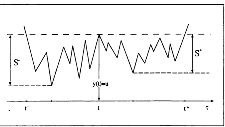
The rainflow cycle counting m ethod was first proposed by Matsuishi and Endo [27] [30] in 1968. The original definition of a rainflow cycle was fairly complicated. It simulated the phenomena of rain dripping down rooftops, and so it was called the “Pagoda Roof m ethod” . Several equivalent versions of the rainflow counting m ethod have evolved [31] [32] [33]. The minor differences which led to the creation of these methods have now been resolved and all give identical cycle counts if the tim e history starts and ends at either the highest peak or the lowest trough. The first alternative and more useful definition was m ade by Rychlik as given below [34].
Definition 1. Let j/(r), —T < r < T, be a load function (Figure 2.3), and suppose it has a local maximum at tim e t with height y{t) = u. Let be the tim e for the first upcrossing after t of the level u, (or = T ii no such upcrossing exists for t < r < T), t~ he the tim e for the first upcrossing before t of the level w, (or t~ = T ii no such upcrossing exists for —T < t < t). Define two ranges at
5+ = max (y(<) - y{r))
t < T < t - r
S~ = max {y{t) - y{T))
t ~ < T < t
The amplitude of a rainflow cycle originating at {t,y{t)) is defined by :
S = m in(5“ , 5'*’)
If the load history is a stationary ergodic tim e signal, a symm etric about t = 0
exists. For this reason, another restriction of S~ > can be applied to the definition. Every cycle counted then should be considered as two cycles with the same amplitude. This modified the definition as [1]:
Definition 2. For a rainflow cycle valued S to exist at a current peak, the signal must have the following configuration as in Figure 2.4:
i). takes the signal forwards ( + v e time) from point 1 to point 2, a distance
y(t)=u
Figure 2.3: R y c h l i k ’s définition for rainfiow cycle
ii). takes the signal forwards from point 2 to point 3, some level at or above point 1.
iii). takes the signal backwards (-ve time) from point 1 to point 4, some level at or below point 2.
iv). takes the signal backwards from point 4 to point 5, some level at or above point 1.
point 1 point 3
points
point 2
point 4
-ve
_ 1 _
time +ve
Figure 2.4: M o d ifie d definition for rainfiow cycle
originally came from a level above point 1 prior to this (given th a t it could go to any level below point 2 during this process).
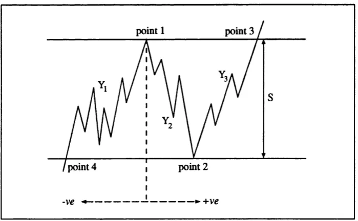
Based on above analysis, a new definition was made by Bishop[35] and is given as below (Figure 2.5):
Definition 3. For a rainflow cycle valued S to be defined from a particular peak the following events must happen:
i). Y\ The signal must have come from a level at least S below the level of point 1 without at any tim e going above the level of point 1 (with any number of extreme points in between).
ii). Y2 The signal must then go from the level of point 1 to some level a
distance S below without at any tim e between going back to the level of point 1 or below the level of point 2 (with any num ber of extreme points in between).
iii). I 3 The signal must then go from the level of point 2 to some level at or above point 1 without at any tim e going back to the level of point 2 (with any number of extreme points in between).
point 1 points
point 2 point 4
-¥ve -ve
Figure 2.5: B i s h o p ’s definition for rain flow cycle
therefore th at large cycles which can be missed very easily by ordinary counting methods is counted by this method. Figure 2.6 shows such an example. Figure 2.6(a) shows a typical strain history. The initial strain excursion, from 0 to A, uses the cyclic stress-strain curve. The strain range 0 to A is plotted on the strain axis, and the stress at point A is calculated from the equation for the cyclic stress-strain curve. Point A is then taken as an origin, the stress range from A to B is then calculated from the hysteresis curve. The actual stress at B then is obtained by subtracting the stress range A to B from the value at point A. By continuing this plotting process until the end of the local strain history, the stress-strain hysteresis history can be derived as shown in Figure 2.6(b).
e
o
(a). A typical local train history
(b). The stress-strain hysteresis loop for strain history (a)
As seen from this stress-strain history, apart from two closed hysteresis loops ranged as E-F and B-C, there exists a large cycle which has the range A-D, which could easily be missed by other counting methods.
2 .4
S to c h a s tic p r o c e s s
2.4.1
G en eral a ssu m p tio n s
The tim e process in general terms can be classified as either d e te r m in is tic or ra n d o m . A determ inistic process can be thought of as one where future states into which the process may fall can be predicted accurately, and with cer tainty. This type of process can generally be expressed explicitly in m athem atical form. Such a process can be either periodic or nonperiodic. A random process is one where the future movements of the process can not be represented by any m athem atical expression with certainty at any particular time.
A s ta tio n a r y random process is one where the statistical properties measured across a set of records, or ensemble, at a particular tim e, are identical with the statistics measured across the ensemble at any other time. In addition to being stationary, the process can be termed e rg o d ic if the statistics measured along any one sample or record are representative of the statistics measured along any other sample. It is much more convenient for statistical com putation if the process has such a property because the statistics can then be obtained from one sample.
2.4.2
P ro b a b ility and m om en ts
If the process is stationary, it can best be described by its probability distribution function P(x) or the probability density function (PDF) p(x), which are indepen dent of tim e t. The moments of the process are defined by its probability density function p(x) as:
/
oo x^p(x)dx -OOThe central moments are similarly defined as:
/
oo (x — x)^p(x)dx-oo
The characteristic function of the process is defined as
<j>{u) = £:{e‘“ } = r e’“> (x )d x (2.7)
J — OO
Thus, the PDF is obtained by applying a Fourier transform ation to the char acteristic function.
p(z) = IT / (2.8)
Z7T V—oo
The characteristic function can be expanded as a MacLaurin series as follows
. 2
+ ... = j=o ^
From Equation 2.7,
i^(«) = <A(0) + i^'(0)u + <!> (0)— + ... = ^ ^ ( « “ )^ + 0 (u " ) (2.9)
çi(")(0) = t" / ” x"p(x)dx =
V—oo
For the situation of more than one random variables, the param eters are defined similarly.
It is obvious that for a general stochastic process, the probability distribution of the process should be described by all the moments of the process. In other words, finite order moments of the process are never enough to fully describe the process. Any truncation causes errors unless the higher order moments can be expressed as functions of lower order moments. The widely used Gaussian distribution with the PDF expressed as
is a good example of where all higher order moments can be calculated from the lower order moments as:
= {n - l)a'^^in- 2 n = 2,4,6,* ••
while the odd moments vanish.
2.4.3
C orrelation fu n ctio n
The cross-correlation function gives a measurement of the amount by which two functions are related to each other. For two random variables x(t) and y(t)^ their cross-correlation function is given by:
The autocorrelation function gives a measurement of the amount by which a signal is correlated with itself. It is defined as the average value of the product
x{t)x{t + r). Provided th at the process is stationary, the value of E[x{t)x{t -f r)] is independent of tim e t and will depend only on the tim e separation r:
Rxx(r) = E[x(t)x{t + r)]
or, alternatively
R x x ( t ) = lim ^ f x ( t ) x { t + T ) d t = R { t ) (2.11)
i —Kx> J —T
2.4.4
Fourier an alysis and sp ectr u m
As well as describing any process in the tim e domain, it can also be described by its Fourier components in the frequency domain [36] [37]. If x(t) is a periodic function of tim e t, with period T, it can be expressed as an infinite Fourier series of the form
OO
x{t) = Û0 + cosLJnt + bk s'munt) (2.12) t=l
where = nu i = n ^ , and the Fourier constants are given by
r 1
ao= - x{t)dt
2
a„ = — / x{t) cos{LOnt)dt n = l,2 ,3 , •••
bn = — x { t ) s m { u j n t ) d t n = 1 ,2 ,3 ,-••
1 Jo
This series expression can also be put in integral form as:
1 .
X(u)) = A{u) - iB ( u ) = — x ( l ) e - “‘d< (2.13)
Z T T J — g o
where A{uj) and B (lj) denote the Fourier constants a„ and bn except th at ao is
put to zero.
An inverse transform would give:
X (w )e'"yw (2.14)
-O O
The most im portant condition for this expansion to hold is th at the function must decay to zero when |i| —» oo, that is,
/
oo \x{t)\dt < oo (2.15)If the process x(t) is random instead of periodic, it can not be represented by a discrete Fourier series. Also, for a stationary process. Equation 2.15 is not satisfied, so th at the Fourier analysis can not be applied to the sample function directly. This difficulty can be overcome by analysing, not sample functions of the process itself, but its autocorrelation function. Provided the mean value of a process is adjusted to zero and the process haa no periodic components, the autocorrelation function does satisfy:
R {t oo) = 0
and then the condition
/
oo \R{T)\dr < oo-O O
is satisfied. The Fourier transform can be applied to R {t).
S{u) = R{T)e~''^''dT (2.16)
27T 2—00
This function is called the spectral density function of the process in radians. It consists of a Fourier transform pair with correlation function as:
/
oo (2.17)-O O
The spectral density function defined in this way is known as the two-sided spectral density function. It gives a “negative frequency” which only makes some sense mathematically. More generally, the one-sided spectral density function is defined to give just positive frequency components and can still give the same mean square value of the process. If the frequency (/) is defined in Hz, it is related to the two-sided spectral density function (in radians w) as:
G{f) = 2 S { f ) = i7rS(üj)
The spectra of the stochastic process X and its derivate X are connected by
Sx(uj) = (2.18)
Similarly,
Sx(uj) = u ‘^Sx{(jj) (2.19)
2.4.5
Fast Fourier Transform
In practical calculations, the transform is generally performed on the discrete tim e series {2^} as:
The one sided Power Spectral Density (PSD) is given by :
Gk{f) = 2L,\\Xk\\^ (2.21)
where, L, = ( N • A t ) and A t is the tim e interval between each tim e point in {Tr}. The PSD defined in this way takes the energy information from the tim e series but discards the phase information.
The computation of the discrete Fourier transform of Equation 2.20 is tim e consuming, especially when TV is big. The Fcist Fourier Transform (FFT ) is there fore generally adopted for this computation. The methodology is th at the work can be performed by partitioning the whole sequence {x^} into a number of shorter sequences. Then, combination of these subsequences together will yield the full DFT of the original sequence.
Suppose th at {x^}, r = 0,1,2, • • • {N — 1) is the sequence where A^is an even number and th at this is partitioned into two shorter sequences { y r } and {zr}
where [36] [38]
Vr = X2r
r = 0 , l , 2 , . . . , ( T V / 2 - l )
2Tr = X2r+1
The D F T ’s of these two short sequences are Tjt and Zk given as:
n = ^ E . e - - )
it = 0 , l , 2 , - - - , ( i V - l ) (2.22)
1 Nl2—\
S
Recombination of Equation 2.20 would give:
. 3v/2-l 7V/2 - 1 (2.23)
r = 0 r = 0
It is found from Equation 2.22 and 2.23 th at
* = 0 , l , 2 , - - - , ( i V / 2 - l ) (2.24)
and {zr} may themselves be partitioned into quarter-sequences, and so on, until eventually the last sub-sequences have only one term each. As Yk and Zk are periodic in k with period N/2, the full com putation is[36]:
' + W ‘z , }
i
. Xt+N/ 2 = l{Yk - W ‘Z , }
in which W =
(2.25)
2.4.6
S ta tistic s in th e freq u en cy d om ain
For the purpose of this thesis the spectrum is characterised by its moments as shown in Figure 2.7. These are actually the weighted sums of the spectrum.
m„ = r
r G ( f ) d f = fj :Gk{fk)Sfk=l
(2.26)
(stress) ^ Hz
Gdf)
frequency, Hz
Figure 2.7: P S D m o m e n t s c a lculation
The even order moments can be calculated from both one-sided and two-sided PSD s. The odd order moments are generally only defined for one-sided PSD ’s.
From Equation 2.18 and 2.26, the zeroth order moment from the spectrum gives the standard deviation of the original process. The 2nd order moment gives the standard deviation of the first order differential process.