Sensor Deployment and Scheduling using
Optimization
V.Blessy Johanal selvarasi A. Aruna Devi
PG Scholar Assistant Professor
Department of Electronics & Communication Engineering Department of Electronics & Communication Engineering Christian College Of Engineering & Technology. Christian College Of Engineering & Technology.
DindigulTamilnadu-624619 India DindigulTamilnadu-624619 India
Abstract
A wireless sensor network (WSN) of spatially distributed autonomous sensors to monitor physical or environmental conditions, such as temperature, sound, pressure, etc. and to cooperatively pass their data through the network to a main location. Wireless sensor networks (WSNs) are known to be highly energy-constrained and each network lifetime has a strong dependence on the nodes battery capacity. As such, the network lifetime has been a critical concern in WSN research. The coverage of sensor nodes deployment becomes one key work that is how to make use of effective node deployment to achieve maximum coverage, it provide good connectivity and energy saving performance. In this project Sensor deployment initially has been done randomly, here Euclidean Minimum Spanning Tree deployment has been proposed. With this algorithm can able to deploy the sensor and compute the coverage matrix in order to get the maximum upper bound network lifetime. Coverage matrix can be achieved by determine the monitoring of sensors. Finally obtained sensor nodes are scheduled using a heuristic so as to achieve the theoretical upper bound of network lifetime. This method helps to prolong the network lifetime. A schedule for notifications on a sensor, rather than disable checking for the sensor all together. The performance can be measured by the calculation of number of sensors, the sensing radius of the deployed sensor and the standard deviation.
Keywords: energy efficient, reliability, flexible, sensor deployment optimization technique
________________________________________________________________________________________________________
I. INTRODUCTION
In wireless sensors have provided us the tool to monitor an area of interest remotely. All one is supposed to do is to deploy these sensors, aerially or manually, and then these sensors which form the nodes of the network gather information from the area under investigation. The information thus obtained is relayed back to the “main server” or “base station” where the information is processed. The base server is sometimes connected to Internet which then relays the processed information via satellite to the main station or control center for further processing and analysis. Very little or no processing is done while information is transferred from nodes. Sensor nodes which constitute the wireless network are autonomous nodes with a microcontroller, one or more sensors, a transceiver, actuators and a battery for power supply.
A wireless sensor network is deployed in one of the two ways: planned and unplanned. In the planned method of deployment a specific number of sensors are placed in strategic points in predetermined manner. Here it should be noted that the area to be monitored can be accessed physically thus the cost is not a factor under such conditions. These nodes are placed using a predetermined algorithm such that the area to be covered is maximized placing less overhead on transmission and battery thereby enhancing the network lifetime. The wireless sensor network faces various issues one of which includes coverage of the given area under limited energy. This problem of maximizing the network lifetime while following the coverage and energy parameters or constraints is known as the Target Coverage Problem in Wireless Sensor Networks . As the sensor nodes are battery driven so they have limited energy too and hence the main challenge becomes maximizing the coverage area and also ensuring a a prolonged network lifetime.
The remaining part of this paper is organized as follows: in section II we describe the details about the previous work of our paper. Section III presents a brief description about TV-Greedy algorithm based on Voronoi partition of the deployment region to reduce the total movement distance of
sensors. Section IV presents simulation results of our proposed method. In section V presents our conclusions.
II. PREVIOUS WORKS
In [5] the system used Voronoi diagrams. It is used to detect coverage holes. After that, sensors are dispatched to cover the detected holes. As a result, the area coverage ratio is improved.Amultiplicatives weighted Voronoi diagram is used to discover the coverage holes corresponding to different sensors with different sensing ranges. However, Voronoi diagram to discover the coverage holes corresponding to different sensors with different sensing ranges. Target coverage can be categorized as simple coverage, k-coverage and Q-coverage.
Voronoi-based methodology for sensor deployment is used which is used to optimize the distance between source and destination. It is a partitioning of a plane into regions based on 'closeness' to points in a specific subset of the plane. That set of points (called seeds, sites, or generators) is specified beforehand, and for each seed there is a corresponding region consisting of all points closer to that seed than to any other. These regions are called Voronoi cells. The Voronoi diagram of a set of points is dual to its Delaunay triangulation.
The balance of power consumption for all sensor nodes in two-dimensional randomly deployed WSNs. A topology construction protocol based on Grid-based WSN is proposed to construct a balanced tree where the total number of nodes in left and right subtrees of the sink node differs at most by one, reducing the delay time for data collection. According to the constructed tree, the number of transmissions of each sensor is derived. To achieve the energy-balanced purpose, two node placement strategies, namely Distance-based and Density-based node placement strategies, are proposed.
Also triangle deployment algorithm to solve simple coverage problem. Triangle deployment algorithm was applied to the dynamic deployment problem in WSNs with mobile sensors on a binary sensing model.Triangle deployment algorithm for sensor deployment problem in irregular terrain.Investigate sensor networks with directional sensing and communication capability and propose a method for deploying sensor nodes with directional sensing range, and subsequent connectivity checking and repairing.In this method which is used to solve only area coverage problem and the number of targets is more compared with number of sensors to be deployed.
In the paper [3] we present a cooperative transmission strategy method is used.The Alamouti space-time code and the maximum ratio combining technique are used for cooperative MISO trans-mission to achieve the spatial diversity gain. These approaches do not aim at solving the energy hole problem and uneven energy dissipation still exists between source nodes and relay nodes, which would cause a reduction in lifetime.
In the paper [4] a novel anonymous on demand routing protocol for wireless mobile ad hoc networks (MANETs). It is used to connect no des in a mobile ad hoc network are vulnerable to both active and passive attacks. A node should not be able to determine whether another node in the network is the sender or the destination of a particular message, a node should not be able to determine whether another node is part of a path between two nodes.
Sensor Scheduling for k-Coverage (SSC) problem which requires to efficiently schedule the sensors, such that the monitored area can be k-covered throughout the whole network lifetime with the purpose of maximizing network lifetime. Here two heuristic algorithms for the SSC problem such as GS and GSAwhich divide the sensors into disjoint/non-disjoint subsets, such that a schedule can be worked out by activating these subsets successively to extend network lifetime, also the fixed/adjustable sensing range issue is considered. Every point in the area needs to be continuously covered (monitored) by at least k sensors. The network lifetime is defined as the total duration during which the whole area is k-covered. k-coverage scheduling problem not achieved the particular requirement such as connectivity and communication range, bandwidth limitation, transmission delay requirement[15].
the other hand, PDND lets the sensors located inside the zones with ground asperities advertise a sensing range that is much lowerthan its “nominal” value, and cause a denser deployment inside the noisy areas.
It is very susceptible to noise and interference, which results in higher inaccuracies of distance estimations [2].
III. PROPOSED METHOD
In our proposed work sensor deployment is done based on Euclidean Minimum Spanning Tree deployment. In Euclidean Minimum Spanning Tree deployment, initially place the sensor randomly. If the sensor not monitored any target then move that sensor to least monitor target. Place the sensor at the center of all target it covers in order to cover new target. Finally calculate the sensor-target matrix for estimating the upper bound of network lifetime. The performance of the process is measured. A simple heuristic to minimize the movement distance of sensors is to minimize the number of sensors that need to move. Actually, after the sensors are deployed, some targets may have already been covered. Denote the set of targets that have already been covered by Tinitcov, anddenote the set of uncovered targets by Tneedcov. Then we have Tneedcov ¼ T n Tinticov. In order to minimize the number of mobile sensors that need to move, we first construct a graph of targets representing whether targets can be simultaneously covered, then find the destinations of mobile sensors by using clique partition.
If a sensor is located in a target’s Voronoi polygon, the sensor is defined as a server to this target, and the target is regarded as a client of its servers. The set of a target’s servers is called that target’s own server group (OSG). The sensor in a target’s OSG that is nearest to the target is called the chief server of the at target, and other sensors are called non-chief servers of the target. Two targets are neighbors if their Voronoi polygons share an edge. For two neighboring targets A and B, the sensor in A’s OSG that is closest to B is called an aid server to B. A target’s candidate server group (CSG) is the union of its own chief server and aid servers from neighbors. For a target, only sensors in its CSG will be dispatched to cover it.The sensors that are used to cover targets in the TCOV problem are referred to as coverage sensors. After the TCOV problem is solved, all the targets are covered by at least one coverage sensor. Besides the coverage of targets in the first stage, another important requirement for a WSN is the connectivity of sensors and the sink, which promises the data transmission. If the sink and the coverage sensors are initially connected, then the connectivity problem is solved; otherwise, we need to study the NCON problem, i.e., how to connect the sink and the coverage sensors.
The basic idea of providing connectivity is to relocate the rest mobile sensors to some locations where they can connect coverage sensors and the sink. Consider a tree-topology, where the sink is the root and all the coverage sensors are the leaf nodes, the goal of NCON is to relocate mobile sensors to new positions as intermediate node to connect the sink and coverage sensors, and the movement of sensor is minimized. From the above analysis, the NCON problem can be solved in two steps. First, we construct an edge length constrained Steiner tree spanning all the coverage sensors and the sink, such that each tree edge length is no longer rc. The Steiner tree is required to minimize the number of sensors that need to move.
NETWORK MODEL
THE TV-GREEDY ALORITHM
THE ECST-H ALGORITHM THE BASIC ALGORITHM
THE ECST ALORITHM
Fig. 3.1: Block diagram of proposed system
the set of targets to be covered (Tneedcov) and the set of mobile sensors to be moved (Srest).It then finds a minimum clique partition on the graph of targets in Tneedcov. For every clique and every sensor in Srest, the potential destination and corresponding movement distance for the sensor to cover targets in that clique is computed. The extended Hungarian algorithm is then used to find which sensor should be moved and to which potential destination so as to cover all the targets. The Basic algorithm minimizes the number of sensors to move, it may increase the total movement distance of sensors.The Target-Based Voronoi Greedy Algorithm is to deploy the nearest sensor to cover the targets that are uncovered. TV-Greedy starts from the generation of targets’ Voronoi diagrams, which divides sensors into independent groups for each target. With assistance of targets’ Voronoi diagrams, we can construct a sensor group for each target, which includes sensors in proximity to this target. Then, the nearest sensor to each target is selected from the target’s group and its neighbors’ group. After that, the selected sensor moves to the corresponding target.
First, we construct an edge length constrained Steiner tree spanning all the coverage sensors and the sink, such that each tree edge length is no longer than r c. The Steiner tree is required to minimize the number of sensors that need to move. Second, we relocate the rest mobile sensors to the generated Steiner points to connect the coverage sensors and the sink. As for the second step, it is actually the special case of TCOV in which the Steiner points are regarded as “target” and the coverage radius is zero. Then for each target we need to dispatch a dedicated sensor to cover it.
With the output SP of the ECST algorithm, the next step is to assign the rest mobile sensors one-by-one to each point in SP with the minimum movement. Since it is actually an assignment problem, it can be solved using the extended Hungarian method. Its computations consist of two parts: the ECST part and the extended-Hungarian part.
Fig. 3.2: Flow diagram of proposed system
The flow diagram describe the sensor nodes and the target coverage areas. Sensors are Randomly deployed, then monitor check the level, there is no sensor means its moves to sorted list, it shows yes means then move to least monitored target. By matrix coverage method sensor are calculated. then moves to sensor sorted nodes, then it place center of the target. then check cover new target, if no coverage it moves to discard section. If there is new coverage until cover another coverge, then sensor are calculated then compute upper bound network lifetime.The advantage of this paper is to robustness when facing network changes and sensor failures.It balances the load of different sensors and prolongs the network lifetime consequently.It is used to find the optimal sensors to move to these points,energy efficient.
IV. RESULTS
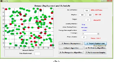
The simulation results shows that sensor deployment and Schedules. the first matlab layout shows the initial state, its coverage region is 1. After the deployment its coverage region is 2. All this deployment, sensing radius is75m, Initial battery power is 100units,energy consumption is 1.
(a)
(b)
The below layout output shows the basic algorithm.the algorithm first finds out the set of targets to be covered (Tneedcov) and the set of mobile sensors to be moved (Srest).It then finds a minimum clique partition on the graph of targets in Tneedcov. For every clique and every sensor in Srest.
(c)
The below diagram shows the tv greedy algorithm output,the first layout shows the intialstate, second layout shows after deployment region, the target-based Voronoi Greedy Algorithm is to deploy the nearest sensor to cover the targets that are uncovered.
(d)
The following algorithm output shows the EX Hungarian outpt. the first layout shows the intial statesecond layout shows the after deployment where its is reach the 6130 level.
(e)
(a)
(b)
Fig. 6: Total movement distance (a) 300m (b) 600-700m
Table – 1 Comparison Table
PARAMETERS EXISTING SYSTEM (BASIC ALGORITHM)
PROPOSED SYSTEM (EX-HUNGARIAN
ALGORITHM)
Total Movement Distance for
400 Mobile Sensor (When
targets are spacing greaterthan
2*rs).
220 90
Total Movement Distance for
100 Mobile Sensor (when
targets are scattered
randomly).
600 700
Total Movement Distance for
40 Targets (When targets are
spacing greater than 2*rs).
790 580
Total Movement Distance for 40 Targets (when targets are
scattered randomly).
680 530
The performance graph will be represented as a chart as following figure 7.
V. CONCLUSION AND FUTURE WORK
Network lifetime is extended by using this method of deploying at optimal locations such that it achieves maximum theoretical upper bound. Then scheduling them so as to achieve the theoretical upper bound and also minimum number of sensor nodes remain active at any time instant. Network lifetime is extended by using this method of deploying at optimal locations such that it achieves maximum theoretical upper bound and then scheduling them so as to achieve the theoretical upper bound. Future work is target coverage achieved by Particle Swarm Optimization Algorithm. PSO is initialized with a group of random particles (solutions) and then searches for optima by updating generations.
REFERENCES
[1] Blumrosen, B. Hod, T. Anker, D. Dolev, and B. Rubinsky, “Enhancing rssi-based tracking accuracy in wireless sensor networks,” ACM Trans. Sens. Netw., vol. 9, no. 3, pp. 1–29,jun. 2013.
[2] Bartolini.N, T. Calamoneri, T. La Porta, and S. Silvestri, “ Mobile sensor deployment in unknown fields”, ACM Trans,INFOCOM2010 pp.471-475,oct 2010.
[3] Dervis Karaboga • Selcuk Okdem • Celal Ozturk Cluster based wireless sensor network routing using artificial bee colony algorithm, ACM Trans.wirelessnetwork.,vol.18,no.7,pp 847-860,oct 2012.
[4] Fu.Z and K. You, “Optimal mobile sensor scheduling for a guaranteed coverage ratio in hybrid wireless sensor networks,” Int. J. Distrib. Sens. Netw., vol. 2013, article no. 740841, pp 1–11,Aug. 2013.
[5] Huang.R, W.-Z. Song, M. Xu, N. Peterson, B. Shirazi, and R.LaHusen, “Real-world sensor network for long-term volcano monitoring: Design and findings,” IEEE Trans. Parallel Distrib. Syst., vol. 23, no. 2, pp. 321–329, Feb. 2012.
[6] Lin.t Chin, P. Ramanathan, K. K. Saluja, and K. Ching Wang, “Exposure for collaborative detection using mobile sensor networks,” in Proc. IEEE 2rd Int. Conf. Mobile Adhoc Sen. Syst., 2005, pp. 743–750.
[7] Liu.B, O. Dousse, P. Nain, and D. Towsley, “Dynamic coverage of mobile sensor networks,” IEEE Trans. Parallel Distrib. Syst., vol. 24, no. 2, pp. 301– 311, Feb. 2013
[8] Lu.M, J. Wu, M. Cardei, and M. Li, “Energy-efficient connected coverage of discrete targets in wireless sensor networks,” in Proc. of 3rd Int. Conf. Netw. and Mobile Comput., pp. 43–52, .
[9] Luo.R.C and O. Chen, “Mobile sensor node deployment and asynchronous power management for wireless sensor networks,” IEEE Trans. Ind. Electron., vol. 59, no. 5, pp. 2377–2385, May 2012.
[10] Somasundara.A.A, A. Ramamoorthy, and M. B. Srivastava,“Mobile element scheduling with dynamic deadlines,” IEEE Trans. Mobile Comput., vol. 6, no. 4, pp. 395–410, Apr. 2007.
[11] Tan.R, G. Xing, J. Wang, and H. C. So, “Exploiting reactive mobility for collaborative target detection in wireless sensor networks,” IEEE Trans. Mobile Comput., vol. 9, no. 3, pp. 317–332, Mar. 20
[12] Wang.G, M. Z. A. Bhuiyan, J. Cao, and J. Wu, “Detecting movements of a target using face tracking in wireless sensor networks,” IEEE Trans. Parallel Distrib. Syst., vol. 25, no. 4, pp. 939–949, Mar. 2014.
[13] Wu.k, Y. Gao, F. Li, and Y. Xiao, “Lightweight Deployment-Aware Scheduling for Wireless Sensor Networks”ACM Trans mobile networks and application, vol.10, no.6, pp.837-852, Jul. 2005.
[14] Yen L.H and Y.-M. Cheng. “Range-Based Sleep Scheduling (RBSS) for Wireless Sensor Networks”, IEEE Trans,vol.48,no.3, pp.411-423,jun 2008. [15] Yingshu Li • Shan Gao. “Designing k-coverage schedules in wireless sensor networks”.IEEE Trans J comb optim vol.15, no.3, pp.847-860,Feb. s2008. [16] Zhuofan liao, jianxein wang, “Minimizing movement for target coverage and network connectivity in mobile sensor networks”,IEEE