ISSN (e): 2250-3021, ISSN (p): 2278-8719
Vol. 10, Issue 1, January 2020, ||Series -IV|| PP 71-81
Multi objective optimization of incremental forming process on
commercially pure Titanium sheet by using Taguchi-Grey and
Regression
Hemant Gurav
1, Firojkhan Pathan
2, Sunil Dambhare
3, Rupesh Patil
4 1Tata Technologies Jamshedpur, India2Department of Mechanical Engineering Dr D.Y.P.I.E.M.R., Akurdi Pune, 3
Department of Mechanical Engineering Dr D.Y.P.I.E.M.R., Akurdi Pune, India 4
Principal NESGI Pune, India
Received 02January 2020; Accepted 16 January 2020
Abstract:
Emerging demand for producing complex shapes on variable materials gives rise to the need for an alternative to the conventional forming process. Incremental forming is a new technique for deforming sheet metals by the application of step-by-step incremental feed to a deforming tool (DT). In this study, commercially pure Titanium sheets were used in incremental forming with an aim to investigate the influences of process parameters such as feed rate, tool diameter, and pitch on the forming of these alloys. By using the Taguchi Method L9 array were finalized for experimentation. Incremental forming was carried out on constant thick pure Titanium sheets in a CNC vertical milling machine. The process was done using a hemispherical shaped tool made of high-speed steel. Optimization of incremental process parameters with the aid of Grey Relational analysis has also been carried out to identify the combinations of the parameters that yield better surface characteristics on the formed sheets. From Grey relational Taguchi Approach it was found that feed rate 2600 rpm, tool diameter 12mm and pitch 0.2 mm are the most promising combination that gives the better surface characteristic. The regression equation is given the optimum solution in the range of operating condition of input parameters. The optimized results of the composite regression equation and regression equation for GRG gives an approximately a similar result.Keywords:
Single point incremental forming, regression. Grey relation, TaguchiI.
INTRODUCTION
In the advance age of manufacturing, Industries requires more complex and aesthetically appealing product which is difficult to achieve through conventional methods. The Conventional forming process is carried out with die and punch which is the main hurdle in automation. The incremental forming process works on a CNC milling machine where complicated external shapes can be formed without use of dies. Due to the development of localized deformation in the case of the conventional forming large amount of stretching takes place. On the other hand, the progressive movement of hemispherical tools gives more flexibility to the manufacturer in case of incremental forming. The wide use of incremental forming is only because of its more flexibility and less tooling cost. This process is generally used in automotive, biomedical and aerospace industries where forming sheet metal used is in batch production [1].
Incremental forming with a partial die, Incremental forming with the full die, Single point incremental forming (SPIF), two-point incremental forming (TPIF) are different types of the Asymmetric Incremental forming used for manufacturing[2,3].Accuracy in the forming angle, as well as surface finish, is still the main concern of Incremental sheet metal forming process [4,5]. The various parameters such as the tool used, plane anisotropy, tool size, and lubrication have great influence on the surface roughness and forming an angle of Incremental sheet metal forming. Incremental Forming on Commercially Pure Titanium (CPTi) sheet shows better surface finish when manufactured by hardened high-speed steel with Molybdenum Disulphide (MoS2) paste as lubricant [6].Tool rotation is one of the influencing parameters on the incremental forming process [7].
Grey relational Taguchi method, Analysis of Variance (ANOVA), and Regression analysis are used to solve optimization problems. Many researchers applied a combination of the Taguchi–Grey relational analysis and improved their experimental results. The Grey relation analysis gives gray relation grade as the single output response parameter which is to be maximized for improvement in performance.[18-22]. Entropy method is used to determine weightage of each output response based on subjective optimization and degree of divergence with respect other output response variable[23-27] which is useful to the conversion of the multi-response problem into single response problem.The single output variable can be analyzed with the help SN ratio and Verified using ANOVA method. The regression analysis is used to determine regression equation of output responses as a function of their input parameters. Also, composite regression model can be useful for multi-output responses [28]
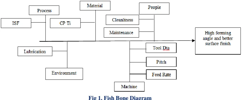
Fishbone diagram represented by Figure No 1 shows various components such as an operating parameter, environment, material etc. which is going to affect the formability of CPTi sheet. Feed rate, tool diameter and pitch are selected as an input parameter for this study.
In the present study, the CPTi sheet is manufactured using the incremental forming process to optimize the input parameter like Feed, Tool Diameter and Pitch for multi-objective optimization Problem (MOOP) on Form angle and surface roughness. Taguchi Method is utilized for experiment design using L9 Orthogonal Array. The Grey relation analysis is implemented to convert a Multi-output variable into the single output. ANOVA is performed to check the fitness model. The confirmation test is carried out to check the repeatability of results. Further regression analysis is performed to find regression equation for Form Angle, Roughness and Grey relation Grade.The Regression equation is optimized for the Composite form angle and Roughness also it is compared with an optimized value of GRG regression model.
This template, modified in MS Word 2007 and saved as a “Word 97-2003Document” for the PC, provides authors with most of the formatting specifications needed for preparing electronic versions of their papers. All standard paper components have been specified for three reasons: (1) ease of use when formatting individual papers, (2) automatic compliance to electronic requirements that facilitate the concurrent or later production of electronic products, and (3) conformity of style throughout a conference proceedings. Margins, column widths, line spacing, and type styles are built-in; examples of the type styles are provided throughout this document and are identified in italic type, within parentheses, following the example. Some components, such as multi-leveled equations, graphics, and tables are not prescribed, although the various table text styles are provided. The formatter will need to create these components, incorporating the applicable criteria that follow.
Fig 1. Fish Bone Diagram
II.
MATERIALS AND METHODS
A. Materials and Chemical Composition
Table No. 1 chemical composition of CPTi
Fe (%) C (%) N (%) H (%) O (%) Others (%) Ti (%)
0.20 0.08 0.03 0.015 0.18 0.4 99.1
Table No 2 mechanical properties of CPTi
Yield strength (MPa) Ultimate tensile strength (MPa) Elongation (%)
230 350 40
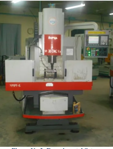
CPTi sheets were cut to the dimensions of 220 x 220 mm. The CNC milling machine is used to perform the Incremental Forming operation with the fixture as shown in Figure No 3. The fixture is designed to hold the sheets as per the normal incremental Forming process standards. A CNC program is written to perform the incremental operation as per required sequence.
Figure No 3: Experimental Set up
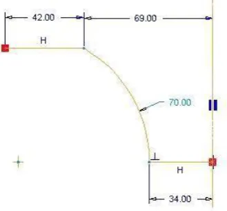
Hemispherical shaped forming tools were fabricated by optical profile grinding. The tools were machined from High-Speed Steel and Silicon Carbide. The geometry of the tool is as shown in Figure No 4
Figure No 4: The geometry of the tool
III.
DESIGNOFEXPERIMENT(DOE)and Pitch with 3 levels for each parameter. The input parameters with levels is illustrated in Table No 3 and L9 orthogonal array is given in Table No 4[13-16]
Table No 3 Design points for DOE
Factors Units Factors
Notation
Levels
1 2 3
Feed RPM A 1200 2600 4000
Tool Diameter mm B 8 10 12
Pitch mm C 0.2 0.75 1.3
Table No 4 L9 Orthogonal Array Exp. No. FeedRate
(A)
ToolDiameter (B)
Pitch (C)
1 1 1 1
2 1 2 2
3 1 3 3
4 2 1 2
5 2 2 3
6 2 3 1
7 3 1 3
8 3 2 1
9 3 3 2
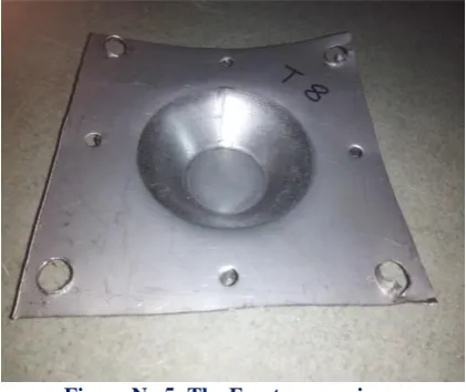
The experiments were performed on CPTi sheet with according to standard procedure with the proper use of lubricants. The Forming is carried out by using Hemispherical Head Tool. The fractured specimen is then studied under standard instrument to measure output response parameters. The Fracture specimen is described in Figure No 5.
Figure No 5: The Fracture specimen
Figure No 6: Formability curve
A. Entropy method[23-28]
AHP method is based on subjective knowledge of output responses and their comparative relationship with respect to each other which entirely depends on the subjective nature of the user. Whereas Entropy Method utilizes Integral information of output response based on their actual values. Each output response shows its disorder degree with other output response. The uncertainty of each response measured with probability theory using following steps which eventually used to find weightage of each output response.
Steps required to solve the Entropy methods are given below
The Normalization of each output response value is calculated by Eq. (1) 𝑃𝑖𝑗 =
𝑥𝑖𝑗
𝑚 𝑥𝑖𝑗2 𝑖=1
(1)
xij is the output response value with respect to j th
output response criteria and ith experiment number. The Entropy value Ej for respective response criteria is calculated with help of Eq. (2)
𝐸𝑗 = −𝑘 𝑃𝑖𝑗ln 𝑃𝑖𝑗, 𝑗 = 1,2, … 𝑛 (2) 𝑚
𝑖=1
Where 𝑘 = 1 ln 𝑚 ;m is number of experiment
The degree of divergence (dj) is determined by Eq.(3)
𝑑𝑗 = 1 − 𝐸𝑗 (3) The weight of respective output response is calculated with the help Eq. (4)
𝛽𝑗 = 𝑑𝑗
𝑑𝑗 𝑛 𝑗 =1
(4).
B. Grey Relation Analysis [17-23]
The Grey relation analysis (GRA) is a method used optimize the multi-objective optimization based on the weight of each output response. GRA converts the multi output into the single output response optimization problem. The steps carried as follows
Normalization of output responses carried out to convert the values of all responses in 0 to 1 range based on the criteria of optimization on output response
For Benefit Criteria (Higher is better) Normalization is carried out by Eq,(5)
𝑦𝑖𝑗 =
𝑥𝑖𝑗 − min 𝑥𝑖𝑗
max 𝑥𝑖𝑗 − min 𝑥𝑖𝑗
(5)
For Cost Criteria (Lower is better) Normalization is carried out by Eq. (6)
𝑦𝑖𝑗 =
max 𝑥𝑖𝑗 − 𝑥𝑖𝑗
max 𝑥𝑖𝑗 − min 𝑥𝑖𝑗
(6)
Where 𝑦 𝑖s normalized value for jth is output response and ith experiment number.
xij is the original output response for the ith Experiment number ofjth output response factor.
ξ𝑖𝑗 =Δ𝑚𝑖𝑛𝑗 − 𝜑∆𝑚𝑎𝑥𝑗 Δ𝑖𝑗 − 𝜑∆𝑚𝑎𝑥 𝑗
(7)
Where
∆𝑖𝑗= 𝑦∗− 𝑦𝑖𝑗 (8)
The 𝑦∗ values depend on the optimization function of the output response. If the output response is to be minimized the ideal value of 𝑦∗is zero otherwise 1.So, Delta values are determined for all the responses by Eq.(8).The Δ𝑚𝑖𝑛𝑗and Δ𝑚𝑎𝑥 𝑗 are the minimum and maximum values of jth output response factor respectively. Generally, 𝜑 value is taken as 0.5.
Gray relation grade for the respective experiment is determined with the help of weights obtained Entropy Method. Grey relation grade (GRG) is calculated with Eq.(9)
𝛾𝑖= ξ𝑖𝑗 × 𝑛
𝑗 =1
𝑤𝑗 (9)
IV.
RESULTS AND DISCUSSION
A. Entropy method
After Normalized output response values are determined for each output response experiment with the help of Eq.1.The Entropy values are then calculated with the Eq.(2) for individual output response. The Degree of divergence value for each output response is determined with Eq. (3).Then the weightage of the same is calculated with Eq. (4).The results are tabulated in Table No 5
Table No 5 Entropy method analysis
Form Angle Roughness
Entropy Value (E) 0.4551 0.4551
Degree of divergence (d) 0.4920 0.4346
Weight (w) 0.5310 0.4690
B. Grey relation Analysis
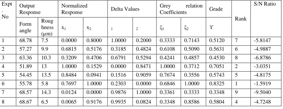
The normalization of output responses is carried out by using Eq. (5-6). As both responses optimized based on cost criteria. The𝛥 values are calculated by using Eq. (8) which is used in Eq. (7) to calculate Grey relation coefficient. As both output responses are equally important.The weightage is taken from obtained Entropy method. The Grey relation grade is obtained with the Eq. (9). The summary of the Grey relation analysis is illustrated in Table No 5.The rank shows the best results among all the experiments. The Experiment Number 6 is having the highest value of GRG i.e. 0.8325 which makes its rank as 1.
The optimum parameter among the 27 possible experiment for 3 level 3 factor design is carried out by S/N ratio which utilized the effect of the interaction of parameters among themselves with the L9 orthogonal array. As discussed earlier GRG is "higher is better criteria" the signal noise ratio for the same is Given Eq. (10). The Table No 6 shows the grey relationship analysis with output responses.
Table No 6 Grey relation Analysis Expt
. No
Output Response
Normalized
Response Delta Values
Grey relation
Coefficients Grade
Rank
S/N Ratio
Form angle
Roug hness (µm)
x1 x2 1 2 ξ1 ξ2 ϒ
1 68.78 7.5 0.0000 0.8000 1.0000 0.2000 0.3333 0.7143 0.5120 7 -5.8147
2 57.27 9.9 0.6815 0.5176 0.3185 0.4824 0.6108 0.5090 0.5631 6 -4.9887
3 63.36 10.3 0.3209 0.4706 0.6791 0.5294 0.4241 0.4857 0.4530 8 -6.8786
4 51.89 13 1.0000 0.1529 0.0000 0.8471 1.0000 0.3712 0.7051 2 -3.0351
5 54.45 13.5 0.8484 0.0941 0.1516 0.9059 0.7674 0.3556 0.5743 5 -4.8175
6 55.78 5.8 0.7697 1.0000 0.2303 0.0000 0.6846 1.0000 0.8325 1 -1.5919
7 68.57 14.3 0.0124 0.0000 0.9876 1.0000 0.3361 0.3333 0.3348 9 -9.5040
𝑆𝑁𝑖 = −10 × log𝑒
1 N
1 𝑥𝑖𝑘2 𝑁
k=1
𝐻𝑖𝑔ℎ𝑒𝑟 𝑖𝑠 𝑏𝑒𝑡𝑡𝑒𝑟 (10)
Where x is the GRG for ith experiment number and N is the total number of repetition. The effect of each level of the input parameter (factor) is summarized with the help of mean S/N ratio plot given Table No 7., which predicts the best operating condition for each input parameter. Figure No 7 plots the mean of S/N ratio for all input parameters corresponds to their respective operating condition.
The analysis shows the most important input parameter is pitch next feed and then Tool parameter. The Table No 7 is also represented in Figure No.7, which illustrate the optimum levels of each input parameter.The optimum parameters are found to be A2B3C1.
Table No 7 S/N Ratio of GRG
Level Feed
Tool
Diameter Pitch
1 -5.852 -6.091 -4.044
2 -3.211 -4.797 -4.181
3 -6.219 -4.394 -7.058
Delta 3.009 1.697 3.014
Rank 2.000 3.000 1.000
Figure No 7: Mean effect plot for SN ratio
C. ANOVA Method
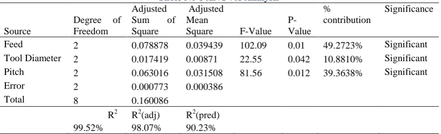
The Analysis of variance method is used to investigate the significance and contribution of each input parameter on the output responses. The ANOVA method uses the variability of output responses, which used for measurement of the sum of squares and mean of square of grey relation grade i.e. output response. The F- test and probability test is carried out to check the significance and contribution of each input parameter on the output responses. The MINITAB software package is used to simulate the experiments. The Grey relation grade is taken as output response which is used for analysis of variance. The results obtained from the ANOVA is illustrated in Table No 8. To determine the significance parameters input parameters Probability Test is used in
which, if the P-Value is less than 0.05 the parameter is said to be significant. As we can see in Table No 7, all three input parameters Feed, Tool Diameter and Pitch are having P values less than the 0.05 which concludes three parameters are significant. The percentage contribution of each input parameter is also shown in Table 7 Which suggests that feed and Pitch contributing more to the model than Tool diameter for this particular model.
The square is 99.52% and squared Adjusted value is 98.07%, which are more than 90% and R-squared Predicted values is 90.23%, which is more than 70 % also the difference between R-R-squared adjusted and R-squared predicted value is less than 20% shows that the model is reasonable agreement.
Table No 8 ANOVA Analysis
Source
Degree of Freedom
Adjusted Sum of Square
Adjusted Mean
Square F-Value P-Value
%
contribution
Significance
Feed 2 0.078878 0.039439 102.09 0.01 49.2723% Significant
Tool Diameter 2 0.017419 0.00871 22.55 0.042 10.8810% Significant
Pitch 2 0.063016 0.031508 81.56 0.012 39.3638% Significant
Error 2 0.000773 0.000386
Total 8 0.160086
R2 R2(adj) R2(pred)
99.52% 98.07% 90.23%
D. Confirmation Test
By using / ratio plot, ideal input process parameter was selected. The S/N ratio prediction model is prepared based on Eq. (11). Prediction model can predict S/N ratio for all input conditions.
𝛾 = 𝛾𝑚+ 𝛾𝑚− 𝛾𝑗 𝑛
𝑗 =1
(11)
Where 𝛾𝑚 is total mean, for the present study 𝛾𝑚 = -5.09411 obtained from Table No 7
𝛾j is mean of the / ratio for selected input parameters, and
n is no. of output responses.
An Initial parameter combination of A1B1C1 has been chosen as it lay at the initial level. The initials testing shows Form angle and surface roughness values to be 68.78 and 7.5 microns which gives GRG -0.52381 and respective S/N ratio -0.561653. The Prediction model is utilized for optimum input parameter i.e. A2B3C1 (feed 2600 RPM, tool diameter 12 mm and Pitch 0.2 mm) which are selected from Figure No 7.The Prediction Model gives S/N ratio value -1.3352 and GRG value from Eq. (10) found to be 0.8575. The authenticity of the prediction model is carried out by confirmatory test as shown in Table No 9, on same input parameter condition which gives Form angle and Surface roughness values 55.43 and 5.9 microns respectively. GRG and SN ratio for the same is calculated to be 0.8431 and -1.4818 which nearer to predicted results. Therefore we can suggest that model is useful for the future experiments.
Table No 9 Confirmation Test
Initial Combination Optimal Combination
Prediction Experimentation
Level A1B1C1 A2B3C1
S/N Ratio -5.8146 -1.3352 -1.4818
Form angle 68.78 55.43
Roughness 7.5 5.9
Grey Relation Grade 0.5119 0.8575 0.8431
E. Regression Analysis
The least square method of regression is used to determine the regression model for individual output responses viz. Form angle and Roughness, Moreover regression equation is built for Grey relation grade. The R2 value, P-value, and error of data is checked to see the fitness equation with actual responses.
a. For form angle, the regression equation is given Eq.(11).
𝐹𝑜𝑟𝑚 𝐴𝑛𝑔𝑙𝑒 = 141.3 − 0.02550 × 𝐹 − 8.150 × 𝑇𝐷 − 36.19 × 𝑃 + 0.00005 × 𝐹2+ 0.3483 ×
Where F=feed in RPM, TD= Tool diameter in mm, and P=Pitch in mm b. For Roughness the regression equation is given Eq.(12)
𝑅𝑜𝑢𝑔ℎ𝑛𝑒𝑠𝑠 = 4.689 + 0.004233 × 𝐹 − 0.07262 × 𝑇𝐷 + 9.519 × 𝑃 + 0.000001 × 𝐹2− 0.02917 × 𝑇𝐷2−
2.920 × 𝑃2− 0.000071 × 𝐹 × 𝑇𝐷 − 0.000087 × 𝐹 × 𝑃 (12)
c. For Grey Relation Grade (GRG) regression equation is given Eq.(13)
GRG = −0.3692 + 0.000591 × 𝐹 + 0.04353 × 𝑇𝐷 + 0.2212 × 𝑃 − 0.0000001 × 𝐹2− 0.000020 × 𝑇𝐷2−
0.2662 × 𝑃2− 0.000006 × 𝐹 × 𝑇𝐷 − 0.000003 × 𝐹 × 𝑃 (13)
R2 values all the regression model are 100%, therefore, we can suggest the equation quite fit the data given. Error obtained after comparing the results of actual and predicted are approximately equal to 0. Further optimization of Form angle with Roughness is carried out together to determined optimized input results as shown figure No 8.With composite desirability of .9254 and optimized results with form angle and roughness as minimization Function are Feed 2444.44, Tool Diameter 12, and Pitch 0.3496.
A similar analysis is carried out GRG regression equation with Maximization function gives optimized results Feed 2529.29 RPM. Tool diameter 12, and Pitch 0.4 as shown in Figure No 9
Figure No 8 Optimization Plot for Form angle and Roughness
V.
RESULTS AND DISCUSSION
The experiments were carried out on three input parameter viz. feed rate (A), tool diameter (B) and pitch (C) to determine the optimum value of two outputs forming angle and surface roughness on commercially pure Titanium (CPTi) sheets.
i. The weights after Entropy method analysis shows more weightage to Form angle i.e. 0.53 to 0.47 for roughness.
ii. Grey relation Analysis converts MOOP into single output problem. The Grey Taguchi analysis shows the best result are obtained for the A2B3C1 (feed rate 2600 RPM, tool diameter 12 mm, and pitch 0.2 mm.) iii. ANOVA analysis shows the contribution of the input parameter to the grey relation grade as Feed rate –
(49.27%), Tool diameter (10.88), and Pitch (39.36). Also
iv. The confirmation test is performed to verify repeatability of results. which shows more improvement results from initial testing
v. The Regression analysis of Form angle, Roughness and GRG give the regression equation. The composite Form Angle and Roughness optimization is carried show the best optimum input parameter setting (Feed 2444.44, Tool Diameter 12, and Pitch 0.3496) which is then compared to optimized values of GRG regression equation (Feed 2529.29 RPM. Tool diameter 12, and Pitch 0.4).
vi. The results obtained after regression analysis are compared to which increase in the value of Tool diameter decrease Form angle and Surface Roughness, Also decrease in value of Pitch decreases the output response which is desirable.
vii. The Nature of feed rate with output response gives optimized value at the middle from 2450 RPM to 2560 RPM according to both regression analysis
REFERENCES
[1]. Thibaud, S., et al. "A fully parametric toolbox for the simulation of single point incremental sheet forming process: Numerical feasibility and experimental validation." Simulation Modelling Practice and Theory 29 (2012): 32-43.
[2]. Khare, U., and M. Pandagale. "A review of fundamentals and advancement in incremental sheet metal forming." IOSR Journal of Mechanical and Civil Engineering (2014): 42-46.
[3]. Daleffe, Anderson, et al. "Analysis of the incremental forming of titanium F67 grade 2 sheet." Key Engineering Materials. Vol. 554. Trans Tech Publications, 2013.
[4]. Liu, Zhaobing, et al. "Modeling and optimization of surface roughness in incremental sheet forming using a multi-objective function." Materials and Manufacturing Processes 29.7 (2014): 808-818.
[5]. Sieczkarek, P., et al. "Wear behavior of tribologically optimized tool surfaces for incremental forming processes." Tribology International 104 (2016): 64-72
[6]. Hussain, Gao, et al. "Tool and lubrication for negative incremental forming of a commercially pure titanium sheet." Journal of Materials Processing Technology 203.1 (2008): 193-201.
[7]. Durante, M., et al. "The influence of tool rotation on an incremental forming process." Journal of Materials Processing Technology 209.9 (2009): 4621-4626.
[8]. Nimbalkar, D. H., and V. M. Nandedkar. "Review of incremental forming of sheet metal
components." Int J Eng Res Appl 3.5 (2013): 39-51.
[9]. Karajibani, Ehsan, Ali Fazli, and Ramin Hashemi. "Numerical and experimental study of formability in deep drawing of two-layer metallic sheets." International Journal of Advanced Manufacturing Technology 80 (2015).
[10]. Atil, Hülya, and Yakut Unver. "A different approach of experimental design: Taguchi method." Pakistan Journal of Biological Sciences 3.9 (2000): 1538-1540.
[11]. Bagudanch, I., et al. "Forming force and temperature effects on single point incremental forming of polyvinylchloride." Journal of materials processing technology 219 (2015): 221-229.
[12]. Bagudanch, I., et al. "Forming force in Single Point Incremental Forming under different bending conditions." Procedia Engineering 63 (2013): 354-360.
[13]. Selvarajan, L., C. Sathiya Narayanan, and R. JeyaPaul. "Optimization of EDM parameters on machining Si3N4–TiN composite for improving circularity, cylindricity, and perpendicularity." Materials and Manufacturing Processes 31.4 (2016): 405-412.
[14]. Manimaran, G., and M. Pradeep Kumar. "Multiresponse optimization of grinding AISI 316 stainless steel using grey relational analysis." Materials and Manufacturing Processes28.4 (2013): 418-423.4
[15]. Onan, M., K. Baynal, and H. İ. Ünal. "Determining the influence of process parameters on the induction hardening of AISI 1040 steel by an experimental design method." (2015).
[16]. Taguchi, Genichi. Introduction to quality engineering: designing quality into products and processes. 1986.
[17]. Montgomery, Douglas C. Design and analysis of experiments. John Wiley & Sons, 2017.
[19]. Hicks, Charles Robert. "Fundamental concepts in the design of experiments." (1964).
[20]. Tarng, Y. S., S. C. Juang, and C. H. Chang. "The use of grey-based Taguchi methods to determine submerged arc welding process parameters in hardfacing." Journal of Materials Processing Technology 128.1 (2002): 1-6.
[21]. Pathan, Firojkhan, Hemant Gurav, and Sonam Gujrathi. "Optimization for Tribological Properties of Glass Fiber-Reinforced PTFE Composites with Grey Relational Analysis." Journal of Materials 2016 (2016).
[22]. Sood, Anoop Kumar, R. K. Ohdar, and Siba Sankar Mahapatra. "Improving dimensional accuracy of fused deposition modelling processed part using grey Taguchi method." Materials & Design 30.10 (2009): 4243-4252.
[23]. Kuo, Yiyo, Taho Yang, and Guan-Wei Huang. "The use of a grey-based Taguchi method for optimizing
multi-response simulation problems." Engineering Optimization 40.6 (2008): 517-528.
[24]. Adalarasan, R., M. Santhanakumar, and A. Shanmuga Sundaram. "Optimization of weld characteristics of friction welded AA 6061-AA 6351 joints using grey-principal component analysis (G-PCA)." Journal of Mechanical Science and Technology 28.1 (2014): 301-307.
[25]. Çalışkan, Halil. "Selection of boron based tribological hard coatings using multi-criteria decision making methods." Materials & Design 50 (2013): 742-749.
[26]. Çalışkan, Halil, et al. "Material selection for the tool holder working under hard milling conditions using different multi criteria decision making methods." Materials & Design 45 (2013): 473-479.
[27]. Yazdani, Morteza, and Amir Farokh Payam. "A comparative study on material selection of
microelectromechanical systems electrostatic actuators using Ashby, VIKOR and TOPSIS." Materials & Design (1980-2015) 65 (2015): 328-334.
[28]. Wakode, Vaibhav R., and Amarsingh B. Kanase-Patil. "Regression analysis and optimization of diesel engine performance for change in fuel injection pressure and compression ratio." Applied Thermal Engineering 113 (2017): 322-333.