Economic Statistical Design of Control Chart using Genetic Algorithm

Economic Statistical Design of

̅

Control Chart

using Genetic Algorithm

Vaisakh P. S.

P. G. Scholar,

Department of Mechanical Engineering,

Mar Athanasius College of Engineering, Kothamangalam, Kerala, India [email protected]

Dileeplal J.

Associate Professor,

Department of Mechanical Engineering,

Mar Athanasius College of Engineering, Kothamangalam, Kerala, India [email protected]

Abstract - Control chart are widely used to establish and maintain statistical control of a process. In other words it is a tool used to monitor the processes and to assure that they remain "in control" or stable. The̅ control chart is preferred most in comparison to any other control chart technique if quality is measured on a regular scale. The design of a control chart involves the selection of the parameters like sample size (n), sampling interval (h), and control limits width (L). The design of a control chart also has an economic aspect as it involves the costs of sampling, inspection, checking for out of control signals, and cost of non-conforming units reaching the consumer. Economic-statistical design is basically a combination of economic and statistical design of control chart. In this type of design, the total cost of maintaining the control chart need to be minimized and at the same time Type-I and Type-II errors are not allowed to exceed their permissible level. In the present work, a genetic algorithm has been developed for the economic design of the

̅

Keywords - Control chart, economic statistical design, expected cost per hour, genetic algorithm.

I. INTRODUCTION

ISO, an international body for formulating standards, has defined quality as degree to which a set of inherent characteristics fulfils requirements. Degree refers to a level to which a product or service satisfies. So, depending upon the level of satisfaction, a product may be termed as excellent, good or poor quality product. Inherent characteristics are those features that are a part of the product and are responsible to achieve satisfaction. Requirements refer to the needs of customer, needs of organization and those of other interested parties (e.g. regulatory bodies, suppliers, employees, community and environment) or it is the expectations that may be stated, generally implied or obligatory (ISO 1802:1994).

Improving the quality of the output is a major factor for a successful and competitive business in the market. Statistical process control (SPC) is one of the best technical tools for improving product and service quality. SPC consists of methods for understanding, monitoring and improving process performance over time (Woodall, 2000). It is now realized that SPC is not just a collection of techniques, but a way of thinking about quality improvement, and it is regarded in many organizations as an important element of Total Quality Management (Caulcutt, 1995).

The main aim behind the idea of control charts is the need for perfection and elimination of non-conforming products. Control chart helps to differentiate between the inherent variation in a process and variation due to assignable causes. The inherent variation in a process is background noise due to several small unavoidable causes. Assignable causes are considerably larger fluctuations when compared to the background noise. Variation from an assignable cause can only be removed from the process through human intervention (Juran and Godfrey, 1998).

Control charts are classified by the type of quality characteristic they are supposed to monitor. Control charts can be broadly classified as control charts for variables and control charts for attributes.

One of the first control charts to receive attention is the ̅ chart, devised by Walter Shewhart. The ̅ chart provides an illustrative example for general control chart theory. The ̅control chart consists of a centre line (CL or μ0), an upper control limit (UCL) and a lower control limit (LCL).

In ̅̅ control chart, the sample mean is compared with the upper and lower control limits of the control chart to decide whether the process is in-control or out-of-control. If a point falls within the upper and lower control limits, the process is referred to as "in control" whereas if it falls outside the control limits, the process is referred to as "out-of control". There are two possible errors: a process can be deemed in-control when in fact the process is out-of-control (Type II error), and vice versa (Type I error). When the process is judged to be out-of-control, there is an attempt to identify the special cause of variation which is called an assignable cause search. (Duncan, 1956)

Generally there are economic design of ̅control chart and economic statistical design of ̅ control chart. In economic design of ̅ control chart, the objective is to reduce the total cost of maintaining the control chart as minimum as possible. It is used to determine the values of various design parameters i.e. sample size (n), sampling interval (h), and control limit coefficient (L) that minimizes total expected cost. The statistical errors associated with control chart are Type-I error and Type-II error. These two errors are cannot be completely eliminated since 100% inspection is not carried out. In economic statistical design, the total cost of maintaining the control chart need to be minimized and at the same time Type-I and Type-II errors are not allowed to exceed their permissible level.

The remainder of this paper is organized as follows: Section II presents the problem description. The proposed genetic algorithm is explained in section III. Result and discussion are presented in section IV and section V gives the concluding remarks.

II. PROBLEM DESCRIPTION

The customer requirements and expectations are becoming increasingly high in terms of quality and cost in the present industrial environment. Accordingly the selection of control chart design parameters like n, h and L becomes a challenging job. The economic statistical design of ̅control chart is considered in this paper to determine the parameters of ̅ control chart.

A. Mathematical model

The mathematical model for economic statistical design of the ̅ control chart is adopted from Rahim and Banerjee cost’s model proposed in 1993. In this model, the failure mechanism belongs to the gamma (λ, 2) distribution, and the sample mean ̅ is normally distributed.

1) The cost model of uniform sampling interval (Rahim and Banerjee, 1993) The objective function of the cost model is expressed mathematically as:

Min F (n, h, L) =

(1)

Subject to α≤ αU, 1-β ≥ PL, and (2)

n ≥ 1 and integer, h ≥ 0, L ≥ 0 (3)

Where E(T) and E(C) represent the expected cycle length and the total expected cost per cycle, respectively. The objective function that the type I error probability (α) and power (1-β) as subjected to the predetermined statistical constraints, including maximum value of type I error (αU) and minimum value of power (PL), is minimized by determining the sample size (n), sampling interval (h), and the control limits (L). This can be expressed mathematically as:

E(T) = h + (αZ0+h)

(

) +

+ Z1 (4)

E(C) = (a+bn+αY+D1h)

( ) + +

+D1 ( ) +W (5)

2) The cost model of non-uniform sampling interval(Rahim and Banerjee, 1993) The objective function of the cost model is expressed mathematically as:

Min F (n, h1, h2, L) =

(7)

Subject to α ≤ αU, 1-β ≥ PL, and (8)

n ≥ 1 and integer, h1 ≥ 0, h2 ≥ 0, L ≥ 0 (9)

Where E(T) and E(C) represent the expected cycle length and the total expected cost per cycle, respectively. The objective function that the type I error probability (α) and power (1-β) as subjected to the predetermined statistical constraints, including maximum value of type I error (αU) and minimum value of power (PL), is minimized by determining the sample size (n), sampling interval (h1, h2, representing the intervals of drawing a sample initially and taking a sample after the first sample over the cycle length, respectively), and the control limits (L). This can be expressed mathematically as:

E(T) = + (αZ0+ )

(

) + + Z1 (10)

E(C) = (a + bn + αY + )

( ) + + + (

) + W (11)

Where α = 2 (-L), β = 1-[ ( √ ) ( √ )] (12)

The parameters of the model are listed below.

Time parameters:

Z0 = the expected search time associated with a false alarm Z1 = the expected search time and repair time if a failure is detected

Cost parameters:

D0 = the expected cost per hour caused by the production of a nonconforming item when the process is in control

D1 = the expected cost per hour caused by the production of a nonconforming item when the process is out of control

W = the expected cost of locating an assignable cause and repairing the process, including the cost of down time Y = the expected cost of false alarms, including the costs of searching and down time if production ceases during the search

a = the fixed cost per sample b = the cost per unit sample

III. METHODOLOGY OF PROPOSED GENETIC ALGORITHM

Genetic algorithms (GA) are the heuristic search and optimization techniques that mimic the process of natural evolution. Simplicity of operation and power of effect are two of the main attractions of the GA approach (Goldberg, 1989). GA can be applied to a wide range of problems (e.g. location, partitioning, and scheduling problems) and GA makes no assumptions about the functions to be optimized.

All that GA requires is a performance measure, some form of population representation, and operators that generate new population members. This general approach can be applied to many combinatorial optimization problems. Hence GA is adapted for the economic statistical design of ̅ control chart in this study. Adaptation is made with respect to chromosome representation, population initialization, crossover operation, and mutation operation in the proposed GA.

1) Mechanism of the proposed genetic algorithm (ESDCC-GA) The proposed genetic algorithm is shown in Figure 1

a. Initialization

Initialize population size (N), crossover rate (CR) and mutation rate (MR) for the proposed genetic algorithm. b. Initial population generation and fitness evaluation

Initial population of size N is randomly generated under a constrained condition for uniform sampling interval and non-uniform sampling interval.

c. Chromosome structure and representation

non – uniform sampling interval is shown in Table 2. The chromosome length (l) is set as equal to number of parameters.

Figure

Figure 1 Proposed genetic algorithm Termination criteria Initial population generation (Parent population) and fitness evaluation

Offspring population generation and fitness evaluation

New population generation (Offspring population + Parent population)

Yes

Final solution (Best chromosome) No

Fitness evaluation Initialize GA parameters

Stop Start

Selection (Roulette wheel selection)

Crossover (Single point crossover)

In the case of sample size, the generated gene value should be discrete, and for sampling interval and control limit, gene value is continuous for each chromosomes.

Gene value of each chromosome is generated using the following equation (Daniel and Rajendran, 2005). Gene= rand ()* (upper_limit - lower_limit) + lower_limit;

Table 1 Chromosome structure for uniform sampling interval scheme

Table 2 Chromosome structure for non-uniform sampling interval scheme

d. Fitness evaluation

Every chromosome in the initial population is evaluated with respect to its fitness function, F = 1/ECT. e. Offspring population generation and fitness evaluation

Offspring populations are generated by applying the following GA operators. 1 Selection - roulette wheel procedure

2 Crossover - single point crossover (based on crossover rate) 3 Mutation - gene wise mutation (based on mutation rate)

The fitness value of each chromosome in the offspring population is also calculated. f. New population generation

The chromosomes in the offspring and parent populations are combined to generate a new population . The best N chromosomes, among the 2N chromosomes are chosen as the surviving chromosomes for the next generation (Parental chromosomes for the next generation).

g. Termination criteria and final solution

The total number of generation is taken as the termination criteria and GA gives the global best solution after termination criteria is satisfied.

IV. RESULTS AND DISCUSSION

A. Economic statistical design of ̅ control chart under uniform sampling interval

In the computational experiment of uniform sampling interval, the population size was set to 80. The crossover probability and mutation probability were set to 0.7 and 0.2, respectively. Parameters are selected based on the pilot study. Generation number is selected based on the convergence analysis of each test problem. For uniform sampling interval, the initial population is randomly generated under the following constrained condition.

1 ≤ n ≤ 3000 (Sample size)

0.1 ≤ h ≤ 100 (Sampling interval)

0.1 ≤ L ≤ 6 (Control limit)

The values of time, cost, Gamma and shift parameters of the example test problem are as follows: Z0 = 0.25 h; Z1 = 1.00 h; D0 = $50.00; D1 = $950.0; W = $1100.00; Y = $500.00; a = $20.00; b = $4.22; δ = 0.50; λ = 0.05; alphaUB = 0.05; and pLB = 0.9. After the experimental study, convergence point of the test problem is identified as 77901th generation and the generation number was set to 80000. The result obtained from ESDCC-GA is compared with the result obtained for same number of solutions (3921017) from PSO (Chih et. al) and it is shown in Table 3. The result shows that EDDCC-GA is better than PSO in terms of minimum ECT and is faster than PSO in terms of elapsed time for uniform sampling interval.

Table 3 Result of uniform sampling interval scheme by ESDCC-GA

Algorithm n h L α 1-β ECT Time (m)

ESDCC-GA 43 4.3879 1.9599 0.05 0.9063 178.0005 29.28 PSO 43 4.3364 1.9602 0.0499 0.9063 178.0085 48.82

B. Economic statistical design of ̅ control chart under non-uniform sampling interval Chromosome, C

g1 g2 g3

n h L

Chromosome, C

g1 g2 g3 g4

In the computational experiment of non-uniform sampling interval, the population size was set to 80. The crossover probability and mutation probability were set to 0.7 and 0.2, respectively. Parameters are selected after conducting the pilot study. Generation number of each test problem under non-uniform sampling interval is selected based on convergence analysis. For non - uniform sampling interval, the initial population is randomly generated under the following constrained condition.

1 ≤ n ≤ 3000 (Sample size)

0.1 ≤ h1 ≤ 100, 0.1 ≤ h2 ≤ 40 (Sampling interval)

0.1 ≤ L ≤ 6 (Control limit)

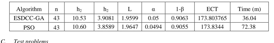
The values of time, cost, Gamma (λ, 2), and shift parameters of the example are as follows: Z0 = 0.25 h; Z1 = 1.00 h; D0 = $50.00; D1 = $950.0; W = $1100.00; Y = $500.00; a = $20.00; b = $4.22; δ = 0.50; λ = 0.05; alphaUB = 0.05; and pLB = 0.9. In the computational experiments of non-uniform sampling interval, convergence point of the test problem is identified as 79946th generation and the generation number was set to 90000. The result obtained from ESDCC-GA is compared with the result obtained for same number of solutions (5062252) from PSO (Chih et. al) and it is shown in Table 4. The result shows that EDDCC-GA is better than PSO in terms of minimum ECT and is faster than PSO in terms of elapsed time for non uniform sampling interval.

Table 4 Result of non-uniform sampling interval scheme

Algorithm n h2 h2 L α 1-β ECT Time (m)

ESDCC-GA 43 10.53 3.9081 1.9599 0.05 0.9063 173.803765 36.04 PSO 43 10.60 3.8589 1.9647 0.0494 0.9055 173.8344 72.38

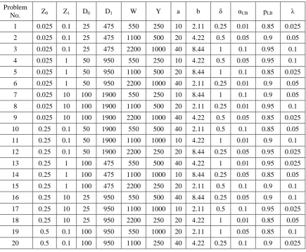
C. Test problems

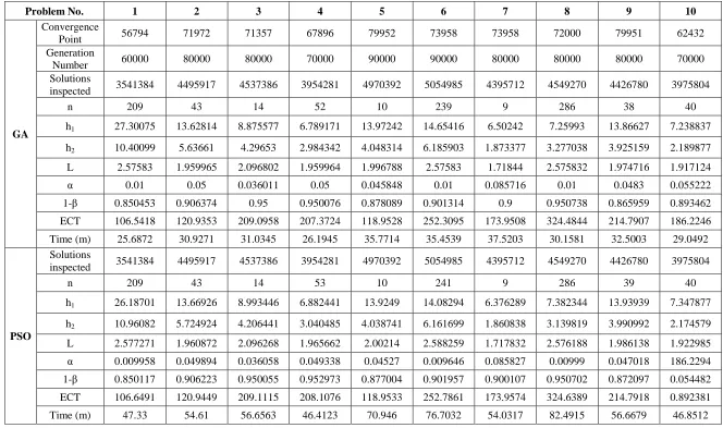
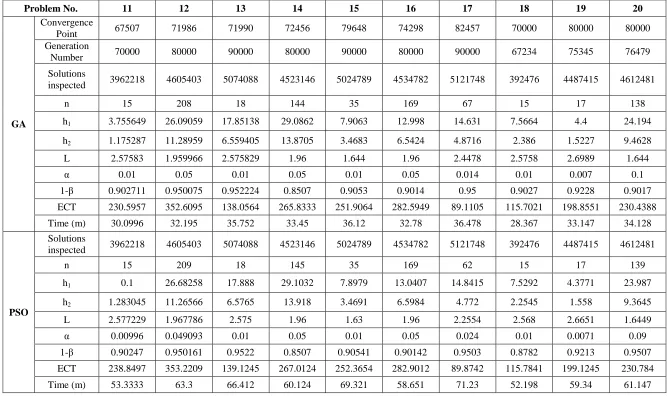
To demonstrate the efficacy of the proposed GA, 20 test problems from literature (Chih et. al) were solved using ESDCC – GA. The test problems considered in this study are shown in Table 5.

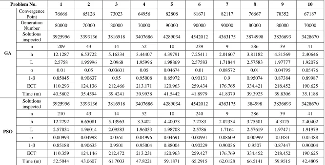
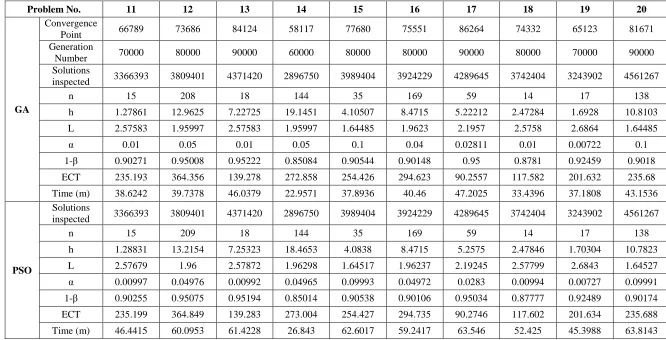
D. Result of test problems

The results of test problems by ESDCC-GA and PSO (Chih et. al) under uniform and non-uniform sampling interval are shown in Table 6 and Table 7 respectively. The result shows that ESDCC-GA takes lesser time than PSO (Chih et. al) for inspecting similar number of solutions in uniform and non-uniform sampling interval. The result indicates that ESDCC-GA is superior to PSO (Chih et. al) in terms of convergence speed for economic statistical design of ̅ control chart.

The proposed GA is better than PSO in terms of minimum ECT and is faster than PSO in terms of elapsed time. Comparing the uniform and non-uniform sampling interval scheme, the expected cost per hour (ECT) is minimum in non-uniform sampling interval scheme.

V. CONCLUSION

This present study aimed to develop a genetic algorithm (ESDCC-GA) for economic statistical design of ̅ control charts under uniform and non-uniform sampling interval. The proposed algorithm is designed to solve the constrained problem, which involves the simultaneous use of continuous and discrete decision variables. To verify the performance of the proposed GA, the numerical example of Rahim and Banerjee (1993) with a Gamma failure mechanism is illustrated in this paper.

Table 5 Test problems

Problem

No. Z0 Z1 D0 D1 W Y a b δ αUB pLB λ

1 0.025 0.1 25 475 550 250 10 2.11 0.25 0.01 0.85 0.025

2 0.025 0.1 25 475 1100 500 20 4.22 0.5 0.05 0.9 0.05

3 0.025 0.1 25 475 2200 1000 40 8.44 1 0.1 0.95 0.1

4 0.025 1 50 950 550 250 10 4.22 0.5 0.05 0.95 0.1

5 0.025 1 50 950 1100 500 20 8.44 1 0.1 0.85 0.025

6 0.025 1 50 950 2200 1000 40 2.11 0.25 0.01 0.9 0.05

7 0.025 10 100 1900 550 250 10 8.44 1 0.1 0.9 0.05

8 0.025 10 100 1900 1100 500 20 2.11 0.25 0.01 0.95 0.1 9 0.025 10 100 1900 2200 1000 40 4.22 0.5 0.05 0.85 0.025

10 0.25 0.1 50 1900 550 500 40 2.11 0.5 0.1 0.85 0.05

11 0.25 0.1 50 1900 1100 1000 10 4.22 1 0.01 0.9 0.1

12 0.25 0.1 50 1900 2200 250 20 8.44 0.25 0.05 0.95 0.025

13 0.25 1 100 475 550 500 40 4.22 1 0.01 0.95 0.025

14 0.25 1 100 475 1100 1000 10 8.44 0.25 0.05 0.85 0.05

15 0.25 1 100 475 2200 250 20 2.11 0.5 0.1 0.9 0.1

16 0.25 10 25 950 550 500 40 8.44 0.25 0.05 0.9 0.1

17 0.25 10 25 950 1100 1000 10 2.11 0.5 0.1 0.95 0.025

18 0.25 10 25 950 2200 250 20 4.22 1 0.01 0.85 0.05

19 0.5 0.1 100 950 550 1000 20 2.11 1 0.05 0.85 0.1

Table 6 Result of test problem under uniform sampling interval scheme

Problem No. 1 2 3 4 5 6 7 8 9 10

GA

Convergence

Point 76666 65126 73023 64956 82808 81671 82117 76667 78352 67187

Generation

Number 80000 70000 80000 70000 90000 90000 90000 80000 80000 70000

Solutions

inspected 3925996 3393136 3816918 3407686 4289034 4542012 4363175 3874998 3836693 3428670

n 209 43 14 52 10 239 9 286 39 41

h 12.1287 6.53722 5.16334 3.44407 4.39791 7.25411 2.01607 3.81182 4.31569 2.40646

L 2.5758 1.95996 2.0968 1.95996 1.98869 2.57583 1.71844 2.57583 1.97777 1.92076

α 0.01 0.05 0.03601 0.05 0.04674 0.01 0.08572 0.01 0.04795 0.05476

1-β 0.85045 0.90637 0.95 0.95008 0.85972 0.90131 0.9 0.95074 0.87384 0.89987

ECT 110.293 124.136 212.466 213.171 120.963 259.434 176.765 334.421 218.452 190.625

Time (m) 40.5602 35.4594 39.4241 39.9938 41.5442 41.8979 41.8379 39.3925 39.8306 35.1188

PSO

Solutions

inspected 3925996 3393136 3816918 3407686 4289034 4542012 4363175 384998 3836693 3428670

n 210 43 14 52 10 240 9 286 39 41

h 12.2792 6.65081 5.13963 3.3402 4.40073 7.2783 2.02334 3.75501 4.3125 2.40402

L 2.57834 1.96014 2.09583 1.96033 1.98708 2.5786 1.7164 2.57619 1.97471 1.91979

α 0.00993 0.04998 0.0361 0.04996 0.04691 0.00991 0.08609 0.00999 0.0483 0.05488

1-β 0.85188 0.90635 0.9501 0.95004 0.88004 0.90229 0.90036 0.9507 0.87447 0.90004

ECT 110.359 124.146 212.472 213.231 120.963 259.427 176.769 334.452 218.452 190.625

Table 6 Result of test problem under uniform sampling interval scheme (Continued)

Problem No. 11 12 13 14 15 16 17 18 19 20

GA

Convergence

Point 66789 73686 84124 58117 77680 75551 86264 74332 65123 81671

Generation

Number 70000 80000 90000 60000 80000 80000 90000 80000 70000 90000

Solutions

inspected 3366393 3809401 4371420 2896750 3989404 3924229 4289645 3742404 3243902 4561267

n 15 208 18 144 35 169 59 14 17 138

h 1.27861 12.9625 7.22725 19.1451 4.10507 8.4715 5.22212 2.47284 1.6928 10.8103

L 2.57583 1.95997 2.57583 1.95997 1.64485 1.9623 2.1957 2.5758 2.6864 1.64485

α 0.01 0.05 0.01 0.05 0.1 0.04 0.02811 0.01 0.00722 0.1

1-β 0.90271 0.95008 0.95222 0.85084 0.90544 0.90148 0.95 0.8781 0.92459 0.9018

ECT 235.193 364.356 139.278 272.858 254.426 294.623 90.2557 117.582 201.632 235.68

Time (m) 38.6242 39.7378 46.0379 22.9571 37.8936 40.46 47.2025 33.4396 37.1808 43.1536

PSO

Solutions

inspected 3366393 3809401 4371420 2896750 3989404 3924229 4289645 3742404 3243902 4561267

n 15 209 18 144 35 169 59 14 17 138

h 1.28831 13.2154 7.25323 18.4653 4.0838 8.4715 5.2575 2.47846 1.70304 10.7823

L 2.57679 1.96 2.57872 1.96298 1.64517 1.96237 2.19245 2.57799 2.6843 1.64527

α 0.00997 0.04976 0.00992 0.04965 0.09993 0.04972 0.0283 0.00994 0.00727 0.09991

1-β 0.90255 0.95075 0.95194 0.85014 0.90538 0.90106 0.95034 0.87777 0.92489 0.90174

ECT 235.199 364.849 139.283 273.004 254.427 294.735 90.2746 117.602 201.634 235.688

Table 7 Result of test problem under non-uniform sampling interval scheme

Problem No. 1 2 3 4 5 6 7 8 9 10

GA

Convergence

Point 56794 71972 71357 67896 79952 73958 73958 72000 79951 62432

Generation

Number 60000 80000 80000 70000 90000 90000 80000 80000 80000 70000

Solutions

inspected 3541384 4495917 4537386 3954281 4970392 5054985 4395712 4549270 4426780 3975804

n 209 43 14 52 10 239 9 286 38 40

h1 27.30075 13.62814 8.875577 6.789171 13.97242 14.65416 6.50242 7.25993 13.86627 7.238837

h2 10.40099 5.63661 4.29653 2.984342 4.048314 6.185903 1.873377 3.277038 3.925159 2.189877

L 2.57583 1.959965 2.096802 1.959964 1.996788 2.57583 1.71844 2.575832 1.974716 1.917124

α 0.01 0.05 0.036011 0.05 0.045848 0.01 0.085716 0.01 0.0483 0.055222

1-β 0.850453 0.906374 0.95 0.950076 0.878089 0.901314 0.9 0.950738 0.865959 0.893462

ECT 106.5418 120.9353 209.0958 207.3724 118.9528 252.3095 173.9508 324.4844 214.7907 186.2246 Time (m) 25.6872 30.9271 31.0345 26.1945 35.7714 35.4539 37.5203 30.1581 32.5003 29.0492

PSO

Solutions

inspected 3541384 4495917 4537386 3954281 4970392 5054985 4395712 4549270 4426780 3975804

n 209 43 14 53 10 241 9 286 39 40

h1 26.18701 13.66926 8.993446 6.882441 13.9249 14.08294 6.376289 7.382344 13.93939 7.347877

h2 10.96082 5.724924 4.206441 3.040485 4.038741 6.161699 1.860838 3.139819 3.990992 2.174579

L 2.577271 1.960872 2.096268 1.965662 2.00214 2.588259 1.717832 2.576188 1.986138 1.922985 α 0.009958 0.049894 0.036058 0.049338 0.04527 0.009646 0.085827 0.00999 0.047018 186.2294 1-β 0.850117 0.906223 0.950055 0.952973 0.877004 0.901957 0.900107 0.950702 0.872097 0.054482 ECT 106.6491 120.9449 209.1115 208.1076 118.9533 252.7861 173.9574 324.6389 214.7918 0.892381

Table 7 Result of test problem under non-uniform sampling interval scheme (Continued)

Problem No. 11 12 13 14 15 16 17 18 19 20

GA

Convergence

Point 67507 71986 71990 72456 79648 74298 82457 70000 80000 80000

Generation

Number 70000 80000 90000 80000 90000 80000 90000 67234 75345 76479

Solutions

inspected 3962218 4605403 5074088 4523146 5024789 4534782 5121748 392476 4487415 4612481

n 15 208 18 144 35 169 67 15 17 138

h1 3.755649 26.09059 17.85138 29.0862 7.9063 12.998 14.631 7.5664 4.4 24.194

h2 1.175287 11.28959 6.559405 13.8705 3.4683 6.5424 4.8716 2.386 1.5227 9.4628

L 2.57583 1.959966 2.575829 1.96 1.644 1.96 2.4478 2.5758 2.6989 1.644

α 0.01 0.05 0.01 0.05 0.01 0.05 0.014 0.01 0.007 0.1

1-β 0.902711 0.950075 0.952224 0.8507 0.9053 0.9014 0.95 0.9027 0.9228 0.9017

ECT 230.5957 352.6095 138.0564 265.8333 251.9064 282.5949 89.1105 115.7021 198.8551 230.4388

Time (m) 30.0996 32.195 35.752 33.45 36.12 32.78 36.478 28.367 33.147 34.128

PSO

Solutions

inspected 3962218 4605403 5074088 4523146 5024789 4534782 5121748 392476 4487415 4612481

n 15 209 18 145 35 169 62 15 17 139

h1 0.1 26.68258 17.888 29.1032 7.8979 13.0407 14.8415 7.5292 4.3771 23.987

h2 1.283045 11.26566 6.5765 13.918 3.4691 6.5984 4.772 2.2545 1.558 9.3645

L 2.577229 1.967786 2.575 1.96 1.63 1.96 2.2554 2.568 2.6651 1.6449

α 0.00996 0.049093 0.01 0.05 0.01 0.05 0.024 0.01 0.0071 0.09

1-β 0.90247 0.950161 0.9522 0.8507 0.90541 0.90142 0.9503 0.8782 0.9213 0.9507

ECT 238.8497 353.2209 139.1245 267.0124 252.3654 282.9012 89.8742 115.7841 199.1245 230.784

REFERENCES

[1] Ben-Daya M. and Rahim M. A., “Effect of maintenance on the economic design of x-control charts”, European Journal of Operational Research, vol. 120 (1), pp. 131–143, 2000.

[2] Cai D. Q., Xie M., Goh T. N. and Tang X. Y., “Economic design of control chart for trended processes”, International Journal of Production Economics, vol. 79, pp. 85 -92, 2001.

[3] Caulcutt R., “The rights and wrongs of control charts”, Applied Statistics, vol. 44 (3), pp. 279–288, 1995. [4] Chen Y. S. and Yang Y. M., “An extension of Banerjee and Rahim’s model for economic design of

moving average control chart for a continuous flow process”, European Journal of Operational Research, vol. 143, pp. 600–610, 2002.

[5] Chen Y. S. and Yang Y. M., “Economic design of ̅ control charts with Weibull in-control times when there are multiple assignable causes”, International Journal of Production Economics, vol. 77, pp. 17–23, 2002.

[6] Chen H. and Cheng Y., “Non-normality effects on the economic–statistical design of ̅ charts with Weibull in-control time”, European Journal of Operational Research, vol. 176, pp. 986–998, 2007.

[7] Chen F. L. and Yeh C. H., “Economic statistical design of non-uniform sampling scheme ̅ control charts under non-normality and Gamma shock using genetic algorithm”, Expert Systems with Applications, vol. 36, pp.9488–9497, 2009.

[8] Chou C. Y., Chen C. H., Liu H. R. and Huang X. R., “Economic-statistical design of multivariate control charts for monitoring the mean vector and covariance matrix”, Journal of Loss Prevention in the Process Industries, vol. 16, pp. 9–18, 2003.

[9] Duncan A. J., “The economic design of ̅ chart used to maintain current control of a process”, Journal of the American Statistical Association, vol. 51, pp. 228-242, 1956.

[10] Girshick M. A., and Rubin H. A., “Baye’s approach to a quality control model”, Annals of Mathematical Statistics, vol. 23, pp. 114-125, 1952.

[11] Lin S. N., Chou C. Y., Wang S. L. and Liu H. R., “Economic design of autoregressive moving average control chart using genetic algorithms”, Expert Systems with Applications, vol. 39, pp. 1793–1798, 2012.

[12] M. A. Rahim, P. K. Banerjee, “A generalized economic model for the economic design of control charts for production systems with increasing failure rate and early replacement”, Naval Research Logistics, vol. 40, pp. 787–809, 1993.

[13] Morteza Behbahani, Abbas Saghaee and Rassoul Noorossana, “A case-based reasoning system development for statistical process control: case representation and retrieval”, Computers & Industrial Engineering, vol. 63, pp. 1107–1117, 2012.

[14] Pei-Hsi Lee, Chau-Chen Torng and Li-Fang Liao, “An economic design of combined double sampling and variable sampling interval X control chart”, International Journal of Production Economics, vol. 138, pp. 102–106, 2012.

[15] Vijaya V. B., Murty S. S. N., “A simple approach for robust economic design of control charts”, Computers & Operations Research, vol. 34, pp. 2001 – 2009, 2007.

[16] Wafik Hachicha, Ahmed Ghorbel, “A survey of control-chart pattern-recognition literature (1991–2010) based on a new conceptual classification scheme”, Computers & Industrial Engineering, vol. 63, pp. 204– 222, 2012.

[17] Weiler H., “On the most economical sample size for controlling the mean of a population”, Annals of Mathematical Statistics, vol. 23, pp. 247-254, 1952.

[18] Woodall W. H., “Conflicts between Deming’s philosophy and the economic design of control charts”, Frontiers in Statistical Quality Control, vol. 3, pp. 242-248, 1987.

[19] Woodall, W. H., “Controversies and contradictions in statistical process control”, Journal of Quality Technology”, vol. 32 (4), pp. 341–378, 2000.

[20] Yan K. C., Hung C. L., “Multi-criteria design of an ̅ control chart”, Computers & Industrial Engineering, vol. 46, pp. 877–891, 2004.