Sensor Location Strategy in Large-Scale Systems
for Fault Detection Applications
Fan Yang and Deyun Xiao
Tsinghua National Laboratory for Information Science and Technology Department of Automation, Tsinghua University, Beijing 100084, P.R,China
Email: {yangfan, xiaody}@tsinghua.edu.cn
Abstract— Fault detection in large-scale systems is conducted by the use of sensors, thus the sensor location influences the performances of fault detection directly. As the scale of systems increases, traditional input-output models may not work well or may even not be applicable. The Signed Directed Graph (SDG) model is used to describe large-scale complex systems and the cause-effect relationships among variables. However, SDG cannot express the dynamic propagation properties when describing the fault propagation phenomena. In this paper, time parameters are taken into account within the branches of an SDG, in order to approximately denote the propagation time of the variable changes in the systems. An SDG constructed this way is called a dynamic SDG. As to sensor location, because of the economic and technical limitations, the number of sensors should be limited while meeting the demands of fault detection. We analyzed the main criteria of the fundamental demand such as reachability, detectability and identifiability of faults in the framework of dynamic SDG, and presented an algorithm to describe the fault propagation process using forward inference and obtained a way to locate sensors. These indices guarantee that the faults can be detected in time and identified from each other. The criteria change when the faults propagate; they are much closer to the reality than those in the framework of a traditional SDG. Some general results, which extend the results obtained in the framework of a traditional SDG, were presented. An algorithm was presented to describe the fault propagation process using forward inference and a way to locate the sensors was obtained. Finally, two examples were used to illustrate the proposed method and results.
Index Terms— sensor location, signed directed graph, large-scale complex system, fault detection
I. INTRODUCTION
In large-scale complex systems, equipments or function blocks are interconnected and the faults in each part may have influence on other parts, i.e. the occurrence of fault in this part may cause some faults in other parts. In order to monitor the state or performance of the system, many sensors are placed everywhere to measure the variables. Theoretically, more sensors located in more places are better for fault detection. But because of economic and technical limitations, we cannot use too many sensors. Given limited resources, we have to choose the most effective and economical way of sensor
location, to detect the fault as quickly as possible (i.e. detectability), distinguish between different faults correctly (i.e. identifiability) and detect the real fault reliably (i.e. reliability).
Firstly, the model, which can express the cause-effect relationships between different variables or faults, needs to be chosen to describe large-scale complex systems. The Signed Directed Graph (SDG) just meets this demand to describe this kind of relationship by using nodes and branches [1]. We can make hazard assessment and fault diagnosis with SDG models [2], and also we can use SDG models to guide the system design such as the sensor location problem. Based on the SDG model, Bhushan,et al.[3-5] have discussed the detectability and
identifiability problems given the sensor location and the corresponding algorithm for locating sensors. Bhushan,et al. [5-7] and Yang, et al.[8] have studied the reliability
problem of fault detection and have proposed some algorithms to choose the sensor location to improve the reliability. However, these methods are all based on a certain static SDG and omit the propagation time of faults. Actually, along with the fault propagation, the properties of fault detection also change. That is to say, detectability and identifiability may change when the fault is propagated along the consistent paths in the SDG model. Thus we should improve the model description by adding the fault propagation time to the traditional SDG. Yang,
et al.[9] have mentioned this idea and have entitled the
time with the name of Fault Revealing Time, and have used it to detect fault origin. In this paper, we call this model the dynamic SDG to emphasize that it shows the dynamic properties of systems, and we use this model to discuss detectability and identifiability problems in fault detection applications.
...
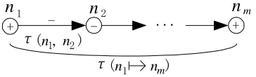
n
1 2
τ
(n1, n2)τ
(n1 nm)+ - - +
Figure 1. Propagation time of a consistent branch and a consistent path.
II. CRITERIA OFFAULTDETECTION
A. The Dynamic SDG and Fault Reachability
In an SDG model, nodes denote variables, and branches denote cause-effect relations. A branch starts from the cause and end at the effect or result. This way, the fault propagation, which is actually a series of continuous propagation from the cause to the effect, is described using the paths composed by nodes and branches. The values of the nodes and branches are all signed by ‘+’, ‘-’, or ‘0’, with the signs of the nodes representing the deviation from the normal value and the signs of the branches meaning the direction of the influence (promotion or depression). The structure and the signs are combined together, so we can determine which branches or paths are consistent. Consistent means the directions of the nodes and branches are consistent with the real case. This is the function of the signs and defines the advantage of the SDG over the use of directed graphs without signs, because faults can be only propagated along consistent branches or paths [10]. Traditional SDGs are static and include no time parameters. Here we take into account the fault propagation time for each branch and form the dynamic SDG. If the variable denoted by the noden1has a direct
influence on the variable denoted byn2, and after a time
period for the fault propagation the fault revealed, then we define this time period τ(n1, n2) as the fault
propagation time betweenn1andn2, as shown in Fig. 1. Obviously, we haveτ(n1,n2)≥0. A path starting fromn1 and ending at nm (denoted as l (n1
nm)) holds the overall fault propagation time τ(n1, nm) which is the summation of timeτ(ni,nj) of each branch in this path, as shown in Fig. 1. Note that this is a simplified treatment, which fits the case of pure propagation delay, but when the dynamic properties are complex, the overall time may slightly decrease due to the effects of intermediate transients [9].Because the nodes in the SDG are classified into two types –variables and fault origins, we denote them asnis andfjs respectively. When a fault occurs, it is propagated along the consistent paths together with the time progress. Definition 1:Starting from the fault node f, after the
timet, the set of nodes affected byfis
( , ) : ( ) ( )
R f t m l f m and f m t ,
wheret is the fault propagation time. If n∈R(f,t), then
we say, nodenis reachable from faultfin time period t.
Obviously, when time proceeds, the set of affected nodes expands, thusR(f,t1)
R(f,t2), ift1<t2.The basic criteria of fault detection are detectability and identifiability that assure the faults are detected and identified from each other. The concepts here are the extension of the concepts in the framework of the SDG.
B. Fault Detectability and Detection Time
A fault should be detected by at least one sensor in a short enough time period. Below is the definition.
Definition 2:If there exist at least one sensor located
in the nodes of R (f, t) (measuring the corresponding
variables), then we say that the faultfis detectable in the
time periodt. The time needed to detect a fault by these
sensors is called the detection timeTD(f).
For each sensor, the time needed to detect a faultfcan
be calculated by shortest path algorithm. Among all these sensors, the shortest time is recorded as TD (f). The
number of nodes with sensors in R (f, t) is called the
degree of detectability.
Based on the traditional SDG, only leaf nodes are needed to consider whether or not to locate sensors [3]. Then we have the following theorem.
Theorem 1:Based on the SDG, disregarding the cases that some variables cannot be measured, sensors need to be located only on the leaf nodes; this being the solution using the least number of sensors.
Proof: According to the weak connection condition, each fault origin has at least one path to the leaf nodes, thus locating sensors on the leaf nodes can meet the detectability criterion. Assume that a sensor location with
n nodes meets the detectability criterion, we can search
an arbitrary path from each node to a corresponding leaf node and put sensors on these nodes, then this new scheme can also meet the criterion, and the number of sensors is no more thann.
Corollary 1:In the framework of dynamic SDG with propagation time, the sensors need to be located on only leaf nodes ofR(f,t).
C. Fault Identifiability and Identification Time
Different faults have different behaviors. Represented in the SDG, the reachable nodes are different. So we must put sensors on these different nodes to identify the different faults. Below is the definition.
Definition 3:If there exist at least one sensor on each of the nodes of R (f1, t) (measuring corresponding
variables), and these sensor nodes are not within the nodes of R(f1,t), in other words, if there are sensors in
the nodes ofI(f1,f2,t) =R(f1,t)∪ R(f2,t)﹣R(f1,t)∩ R
(f2,t), then we say that the faultsf1andf2are identifiable
in the time period t. The time needed to identify two
faults by these sensors is called the identification time TI
(f1,f2).
Detectability and identifiability are two independent concepts. We can understand easily, when two faults are both detectable, they may not be identifiable. On the other hand, identifiability does not imply detectability generally, because we can place only one sensor to identify them too. But usually we assume that only when the faults are detectable, they can be considered for identifiability. Thus the identifiability condition is stronger. In Definition 3, I (f1,f2,t), for two identifiable
identifiability. Besides, we have
Proposition 1:TI(f1,f2)≥max{TD(f1),TD(f2)}.
Proposition 2:The number of elements inI(f1,f2,t) is
not necessarily increasing monotonically with timet.
It should be noted that the signs of the nodes and branches can help to identify different faults because some sensors are not only able to activate the alarm, but also indicate the direction of the departure from the normal values. For this case, we could change a node into two, one shows the higher reading, another shows the lower reading [11]. Then the above definition and the following rules can be applied.
D. Detectability and Identifiability with Multiple Faults
Sometimes we also need to deal with the case of multiple simultaneous faults, it can be dealt by node set transformation. Of course, the probability of this case is extremely small, so we usually omit this case.
Here we take two faults as an example. If the faultsfi andfjoccur at the same time, their reachable node set is
Ri∪ Rj, so we can take these Cn2 node sets to be considered besides the sets of Ri, then the problem is transformed into the detectability and identifiability problems with a single fault.
Obviously, if each fault can be identified, but when several faults occur at the same time, they are not assured to be identified. How about the inverse proposition?
Theorem 2:If the case ofnsimultaneous faults can be
identified, then the case of less thannsimultaneous faults
can be also identified.
Proof: Assume that the case of 2 simultaneous faults can be identified, then for arbitraryi,j,kandl, we have Ri∪ Rj≠ Rk∪ Rl. Thus for arbitraryi, andj, we haveRi≠
Rj, otherwise, assume that there existsiandj, so thatRi≠
Rj, then (Ri∪ Rk) – (Rj∪ Rk) = (Ri –Rj) ∪ Rk = . Therefore, each fault can be identified. Similarly, the case of multiple simultaneous faults are correct.
III. GENERALCHOICE OFSENSORLOCATION
A. Practical Design Method of Sensor Location
The purpose of the sensor location problem is to choose sensors and design the sensor location to meet the demands of fault detection. With the exception of the reliability problem, here we deal with the detectability and identifiability problems. There are usually two requirements referring to sensor location: (1) Given limited time, locate properly the least sensors to meet the demands. Bhushan,et al.[3,4] have proposed algorithms
for the SDG without propagation time. It is similar when we introduce the time parameters. (2) Given the maximum number of sensors, select a location strategy to realize the best performance of fault detection with the shortest time. The above two problems are the two aspects of one problem; they can be integrated into one algorithm.
In the framework of the static SDG, the problem can be solved directly. But in the framework of dynamic SDG, the conditions are complex. The arising times of various
faults are stochastic, and the effects of multiple faults may mix, so it is hard to analyze all the cases of fault propagation or even solve the sensor location problem in advance. In real cases, the sensor location problem is embedded in the forward inference process. Taking the inference algorithm for dynamic Bayesian network [12], the inference method and realization method for the sensor location in the framework of dynamic SDG is presented as follows.
1. Add fault nodefito the evidence node setEand the reachable node setRi. Set the inference system time Tsys to zero.
2. Check if the evidence node set is empty. If it is empty, then go to the end, otherwise go on.
3. From the evidence nodes, choose the nodes in the reachable node set for one forward step, and add them to the reachable node set RE of the evidence nodes. Meanwhile, update their detection time TD(fi) (detection time of the starting node of the branch plus the propagation time on the branch).
4. From the nodes inRE, choose one with the shortest detection time Tk and the nodes to be updated, NTk , at
timeTk.
5.Tsys=Tsys+Tk. Make forward inference from all the nodes in NTk for one step.
6. Add NTk to the evidence node setE and reachable
node setRi.
7. If an evidence node whose one-step reachable nodes are all updated, then delete this node fromE.
8. Placing sensors in the reachable node set Ri can assure the detectability of fault i, and placing sensors in Ri∪ Rj ﹣Ri∩ Rj can assure the identifiability of fault i andj.
9. If a new fault has occurred, then add its corresponding node to the evidence node set E, and set Tsysas the current time. Go to 2.
Note that the treatment in step 3 is not accurate because the detection time is just approximate. So we often increase the threshold of the degree of detectability and identifiability to assure performance is optimal. And if the reliability demands are considered, we need optimization algorithms.
With this algorithm and its extension, we can decide the sensor location, together with the forward inference, at any cases of fault occurrence. Under different cases, the sensor location is also different, but there are some elementary rules.
B. Some Results Based on the Structure Characteristics of the SDG
In engineering practice, there are some rules to assist the sensor location design.
Rule 1:IfR(f1,t) andR(f2,t) are not empty and have
no intersection, then from each set, choose one node with the shortest propagation time from the faultsf1andf2.
As shown in Fig. 2(a), faultsf1andf2have no influence
f1 f2 f1 f2 f1 f2
n1 n2
n1 n2 n
1 2 3 4
(a) (b) (c)
Figure 2. Several common cases of fault propagation and their SDGs.
(a)
(b)
(c)
Figure 3. Several common cases of fault propagation and their SDGs. Rule 2:If the setsR(f1,t) andR(f2,t) are not empty,
and there is a time t subject toR (f1,t) ≠ R (f2,t), then
from the setsR(f1,t)﹣R(f1,t)∩ R(f2,t) andR(f2,t)﹣
R (f1, t) ∩ R (f2, t), choose one node with the shortest
propagation time from the faultf1andf2.
In all the cases, the setsR(f1,t)﹣R(f1,t)∩ R(f2,t)
andR(f2,t)﹣R(f1,t)∩ R(f2,t) do not intersect; so Rule
1 can be applied.
Rule 3:If the reachable nodes of faultf1andf2are the
same, then we can only locate sensors to identify the two faults temporarily.
As shown in Fig. 2(b), the reachable nodes of faultsf1
andf2aren1andn2. The propagation time of each branch
has been labeled beside the branch, the unit of which is minute. Assume the fault f1 andf2occurred at the same
time when the system time is zero. Between the time 1 to 3, faults have only been propagated to n1, now the two
faults can be identified. But after the time 3, faults have been propagated to n1 and n2, then they cannot be
identified any more.
Rule 4:If there is a node n∈R (f1,t), and for all the
timet,n∈R(f2,t), then the nodencan be used as sensor
node to identify the faultf1andf2.
As shown in Fig. 2(c), node n can assure the
identifiability of faultf1andf2at any time.
IV. CASESTUDY
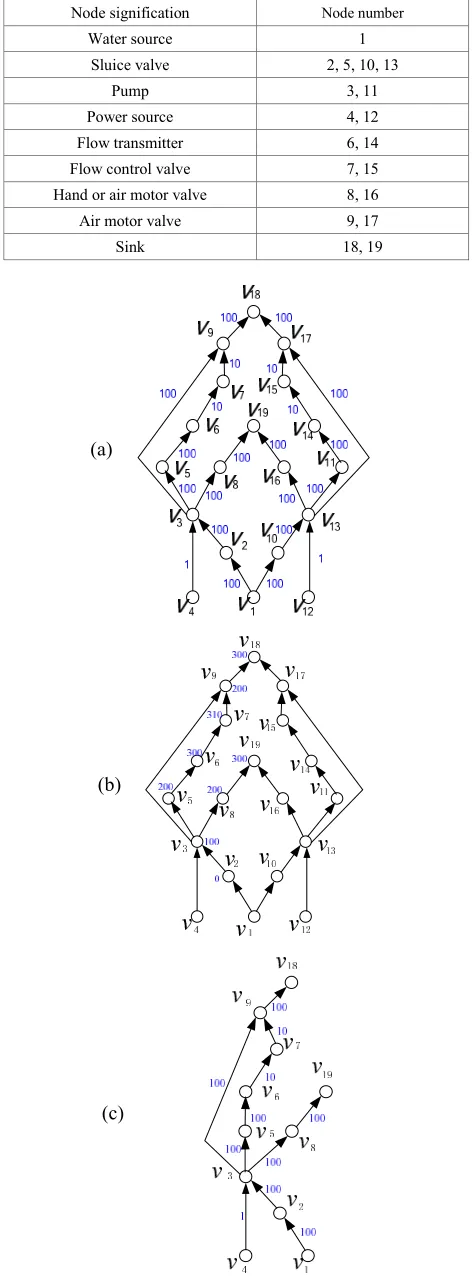
A. Pump System
First we give a simple example, a pump system with 19 elements [13], to illustrate the above concepts and methods. The meaning of the nodes in this system is shown as Table I, and the corresponding dynamic SDG is shown as Fig. 3(a) with the fault propagation time on each branch. According to the above algorithms, we can obtain the fault propagation process of each fault. For example, the fault revealing time of all the variables caused by the faultv2is shown in Fig. 3(b).
The reachable node sets of v4andv12do not intersect
before 201 seconds, thus the two faults are identifiable. After 201 seconds, however, the sensors located on v18
andv19can also detect faults so that they cannot identify
the two faults, but all the other nodes in the fault reachable sets can be used to identify them.
Due to the symmetry of the SDG, we only use half of it, shown as Fig. 3(c). If faults occur on v1 and v4
simultaneously, then their fault reachable sets are the same except v2 and themselves, thus we can locate sensors on v2 and v3. After 100 seconds, the two faults
TABLE I.
NODESIGNIFICATIONS OF THEPUMPSYSTEM Node signification Node number
Water source 1
Sluice valve 2, 5, 10, 13
Pump 3, 11
Power source 4, 12
Flow transmitter 6, 14
Flow control valve 7, 15
Hand or air motor valve 8, 16
Air motor valve 9, 17
PIC-04
LIC-02 FR-04
LIC-01
FI-08
FR-01 FI-03
TIC-01 PIC-01
AI-01
PI-03 PI-05
FI-06 FR-02
PIC-02
PIC-03 FR-07
TI-07
FM FH
FL
FG
Figure 5. The simplified SDG of a boiler system. Figure 4. The main flow chart of a 65 tonnes per hour boiler.
can be identified, and the detection time of v2 is 100 seconds whilev3is only 1 second.
Consider the simultaneous fault ofv3andv5, if they are
both unmeasurable, then they cannot be identified because their downstream nodes are exactly the same. However, if we consider the fault propagation time, then they can be identified according to the detection time of
v6, v7,v9andv18, in which the difference ofv6and v7 is
the propagation time fromv3tov5and the difference ofv9 andv18is the propagation time fromv3tov5.
B. Boiler System
Further, we choose a 65 tonnes per hour steam boiler system as a more actual example that is widely used in power and petrochemical enterprises, and realize the operation in both normal and abnormal conditions by a simulation software ─ Personal Simulator [14] whose interface of the main flow chart is shown as Fig. 4. The simplified SDG of the system is shown as Fig. 5 which
only describes the relationships between the key variables including inlet flow rate of the boiler FR-01, outlet flow rate of the superheated steam FR-02, flow rate of the cooling water FI-03, flow rate of the softened water FR-04, flow rate of the smoke FI-06, flow rate of the fuel oil FR-07, flow rate of the deoxidizing water to be catalyzed FI-08, pressure of the hearth PI-03, pressure of the smoke at the exit PI-05, oxygen percentage of the smoke AI-01, pressure of the main steam PIC-01, pressure of the high pressure gas PIC-02, pressure of the liquid hydrocarbon PIC-03, pressure of the deaerator PIC-04, water level of the top steam drum LIC-01, water level of the deaerator LIC-02, temperature of the overheated steam TIC-01, temperature of the hearth TI-07, flow rate of the inlet gas FG, and the flow rate of the high, medium and low pressure gas denoted by FH, FM and FL respectively [15].
nodes from their downstream nodes because they are independent of each other. Faults on FR-04 and FI-08 cannot be identified putting sensors on the nodes of this SDG, because their downstream nodes are exactly the same. But if we put a sensor on LIC-02 and consider the direction of the deviation, they can be identified. Besides, because the propagation times from them to LIC-02 are different, so maybe we identify them in a short time period. According to Rule 4, in order to identify FR-02 and FH, a sensor can be placed on LIC-01. There are many similar examples to this case.
If the algorithm we presented is applied, the above results can be also obtained. And if we omit the propagation time, the sensor location can be decided aiming to the common faults; this is the simplified case of this method, and the result is as same as the result from the traditional method.
V. CONCLUSION
The SDG has its advantages in the description of large-scale complex systems, but the qualitative and static properties limit its application. In the real engineering systems, quantitative and dynamic properties are shown as propagation time, gain, trend, probabilities and so on. This paper introduced the propagation time and obtained the dynamic SDG which we can use to analyze the principles of fault propagation. Also, because the dynamic propagation of faults is considered, the sensor location we get in this way is closer to reality, and we can accomplish it according to the demands of detectability, identifiability and other criteria. When there are many kinds of fault origins, and the probability of multiple faults are high, we can make forward inference to do the analysis to deal with the various possibilities. Of course, because of the incomplete and even incorrect information, this method is not accurate enough, but in most cases, it can meet users’demands and help with the system design.
The dynamic SDG we used here is very rough for it just introduces the time element but not refer to other dynamic properties. The real dynamic systems should be modeled in more accurate ways, and the sensor location method should be researched upon this model. Gentil et al [16] proposed a representation method of temporal
phenomena by transfer functions and their operations. This may be a better or preciser model for dynamic system and may be transformed into dynamic SDGs.
ACKNOWLEDGMENT
The work was supported in part by a grant from the National High Technology Research and Development Programme of China (No. 2003AA412310) and National Natural Science Foundation of China (No. 60736026). The authors gratefully acknowledge the financial aid for this research.
REFERENCES
[1] M. Iri, K. Aoki, E. O’shima, and H. Matsuyama, “An algorithm for diagnosis of system failures in the chemical
process,”Computers and Chemical Engineering, vol. 3, no. 1-4, pp. 489–493, 1979.
[2] F. Yang and D. Xiao, “Review of SDG modeling and its application,”Control Theory and Applications, vol. 22, no. 5, pp. 767–774, October 2005.
[3] R. Raghuraj, M. Bhushan, and R. Rengaswamy, “Locating sensors in complex chemical plants based on fault diagnostic observability criteria,”American Institute of Chemistry Engineering Journal, vol. 45, no. 2, pp. 310– 322, February 1999.
[4] M. Bhushan and R. Rengaswamy, “Design of sensor network based on the SDG of the process for efficient fault diagnosis,” Industrial and Engineering Chemistry Research, vol. 39, no. 4, pp. 999–1019, March 2000. [5] M. Bhushan and R. Rengaswamy, “Design of sensor
location based on various fault diagnostic observability and reliability criteria,”Computers and Chemical Engineering, vol. 24, no. 2-7, pp. 735–741, July 2000.
[6] M. Bhushan and R. Rengaswamy, “Comprehensive design of a sensor network for chemical plants based on various diagnosability and reliability criteria— 1. Framework,” Industrial and Engineering Chemistry Research, vol. 41, no. 7, pp. 1826–1839, April 2002.
[7] M. Bhushan and R. Rengaswamy, “Comprehensive design of a sensor network for chemical plants based on various diagnosability and reliability criteria— 2. Applications,” Industrial and Engineering Chemistry Research, vol. 41, no. 7, pp. 1840–1860, April 2002.
[8] F. Yang and D. Xiao, “Reliability description of fault detection and optimization algorithm of sensor location,” Journal of Applied Sciences, vol. 24, no. 2, pp. 125–130, March 2006.
[9] F. Yang and D. Xiao, “Approach to fault diagnosis using SDG based on fault revealing time,”inProceedings of the 6th World Congress on Intelligent Control and Automation, Dalian, 2006, pp. 5744-5747.
[10] M. Iri, K. Aoki, E. O’shima, and H. Matsuyama, “A graphical approach to the problem of locating the origin of the system failure,”Journal of the Operations Research, vol. 23, no. 4, pp. 295–311, December 1980.
[11] N.A. Wilcox and D.M Himmelblau, “The possible cause and effect graphs (PCEG) model for fault diagnosis— I. Methodology,”Computers and Chemical Engineering, vol. 18, no. 2, pp.103–116, February 1994.
[12] Y. Hu, “The research and application of cyclic and dynamic Bayes network,” Ph.D dissertation, School of Information Engineering, University of Science and Technology Beijing, Beijing, China, 2001.
[13] K. Masasumi, M Satoshi M, and S Sadanori, “Fault location using digraph and inverse direction search with application,”Automatica, vol. 19, no. 6, pp. 729-735, 1983. [14] C. Wu, “Modeling and simulation of 65t/h steam boiler for
operation analysis,”Boiler Technology, vol. 33, no. 9, pp. 1–6, September 2002.
[15] F. Yang and D.Y. Xiao, “Approach of building qualitative SDG model in large-scale complex systems,”Control and Instruments in Chemical Industry, vol. 32, no. 5, pp. 8–11, October 2005.
Fan Yangwas born in Beijing on 25 February 1980. He got his BSc degree in Automation and Doctorate in Control Science and Engineering in Department of Automation, Tsinghua University, Beijing, China in 2002 and 2008. His major field of study includes fault analysis and hazard assessment.
He is now a Postdoctoral Fellow in Tsinghua University and has published more than 10 papers in academic journals as Control Theory and Applications, Control and Decision, etc, and international conferences as IFAC World Congress and IEEE SMC. His current research interest is the system modeling, fault analysis and hazard assessment based on signed directed graphs.
Dr. Yang is a member of IEEE and IEICE. He obtained the Young Research Paper Award issued by IEEE Control Systems Society Beijing Chapter in 2006.
Deyun Xiaowas born in Fujian, China on 12 August 1945. He graduated from Tsinghua University, Beijing, China in 1970 and has been working in Department of Automation, Tsinghua University. His major field of study includes fault diagnosis, system identification, hybrid systems, sensor data fusion, computer control systems, urban intelligent transportation systems, space robot system, real-time database systems, and computer integrated manufacturing systems.
He is a Professor in Department of Automation, Tsinghua University and has published more than 100 academic papers and several books like Process Identification (Beijing: Tsinghua University Press, 1988) and so on.