Investigation of the Characteristics of the Zeros of the Riemann Zeta Function in the Critical Strip Using Implicit Function Properties of the Real and Imaginary Components of the Dirichlet Eta Function

(1)

Investigation of the Characteristics of the Zeros of the

Riemann Zeta Function in the Critical Strip Using

Implicit Function Properties of the Real and Imaginary

Components of the Dirichlet Eta function

Andrew Logan1∗

1_{4 Easby Abbey, Bedford MK41 0WA, UK}

This paper investigates the characteristics of the zeros of the Riemann zeta function (of s) in the critical strip by using the Dirichlet eta function, which has the same zeros. The characteristics of the implicit functions for the real and imaginary components when those components are equal are investigated and it is shown that the function describing the value of the real component when the real and imaginary components are equal has a derivative that does not change sign along any of its individual curves - meaning that each value of the imaginary part of s produces at most one zero. Combined with the fact that the zeros of the Riemann xi function are also the zeros of the zeta function and xi(s) = xi(1-s), this leads to the conclusion that the Riemann Hypothesis is true.

Keywords: riemann zeta; dirichlet eta; implicit function; harmonic addition; analysis; critical strip; zeros

I. INTRODUCTION

This paper investigates one of the key unresolved questions arising from Riemann's original 1859 paper regarding the distribution of prime numbers ('Ueber die Anzahl der Primzahlen unter einer gegebenen Grősse' - translation in Edwards) - the nature of the roots of the Riemann xi function ( 'One finds in fact about this many real roots within these bounds and it is very likely that all of the roots are real' - referring to the roots of the Riemann Xi function).

This paper starts in section 2 from Riemann's original definition of ζ(s) and ξ(s) and notes the implications of ξ(s) in power series form for the roots of ξ(s) and therefore of ζ(s).

Section 2 also highlights the characteristics of the real and imaginary components of ζ(s) and investigates the behaviour of the function re(ζ(s))=im(ζ(s)) for a specific example, showing the unlikely nature of there being two zeros of the entire function for a fixed value of the imaginary part of s.

Section 3 looks more formally at the Dirichlet eta function (η(s)) which has the same zeros as ζ(s). The implicit function described by the real component being equal to the imaginary component of η(s) is established as a series and substituted into the function describing the value of the real component when the real and imaginary components are equal

(recognising that a necessary condition for a zero of η(s) is a zero of the real component of η(s). Using the Harmonic Addition Theorem the derivative of the real component of η(s) when the real component is equal to the imaginary component is shown not to change sign along any of its individual curves. This leads to the conclusion that any fixed imaginary component of s can produce at most one zero for the real component of η(s).

Section 4 develops the implications of the earlier investigations, leading to the conclusion that the Riemann Hypothesis is true.

II. PRELIMINARY -

OBSERVATIONS OF THE CHARACTERISTICS OF THE

REAL AND IMAGINARY COMPONENTS OF THE RIEMANN ZETA FUNCTION HIGHLIGHTING WHEN THEY

HAVE THE SAME VALUE

A. Riemann Zeta Function and Riemann Xi Function Definitions

(2)

ζ(s)= ∑ 1

𝑛𝑠

𝑛 =∏𝑝_1−𝑝1−𝑠 (Absolutely convergent for Re(s)>1)

Riemann then extends the zeta function analytically for all s and defines the xi function (which has the same zeros as the zeta function) and shows that it can be written as a power series (Edwards, 2001):

ξ(s)=∑ 𝑎2𝑛(𝑠 − 1 2)

2𝑛 ∞

𝑛=0 where

𝑎2𝑛= 4 ∫ (_𝑑𝑥𝑑 (𝑥 3

2𝜑′(𝑥)) 𝑥− 1 4 𝑙𝑜𝑔𝑥

2𝑛 22𝑛_(2𝑛)! ∞

1 )𝑑𝑥

Now, using Riemann's s = 1/2+it and defining t=(a+bi), then (s-1/2) = it = (ai-b), and:

ξ(s)=∑∞𝑛=0𝑎2𝑛(𝑎𝑖 − 𝑏)2𝑛

Note that the functional equation of the zeta function is equivalent to ξ(s)=ξ(1-s) (Edwards p16). This, combined with the fact that any complex root of the power series will also

have the complex conjugate of that root as a root, means that if (b+ai) is a root of ξ(s), then so are all of (b-ai), (-b+ai) and (-b-ai). This, in turn, means that (1/2+b +ai), (1/2+b -ai), (1/2-b +ai) and (1/2-b -ai) are all roots of ζ(s).

For convenience, the real part of s (equivalent to (1/2 +/- b)) will be referred to as σ in the rest of this paper.

B. Riemann Zeta Function Real and Imaginary Component Characteristics Observations

Analytic extensions of the function valid for all s are well documented and have been used to make useful (numerical) applications for calculating ζ(s). One of these numerical applications (from matlab) was used to create the 2 figures following, before we look at a more formal approach.

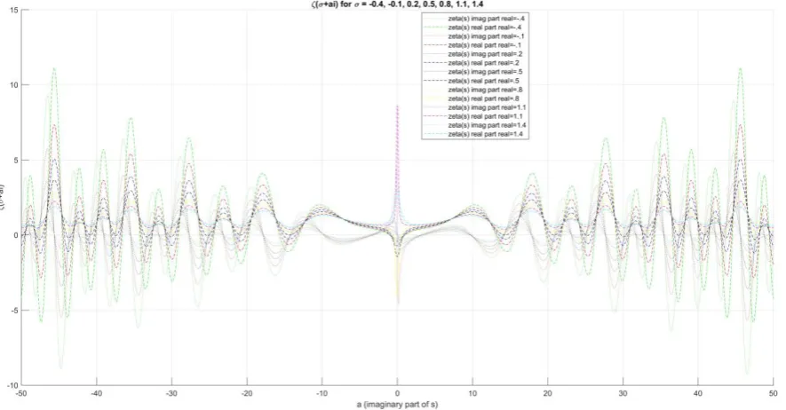
Observing the characteristics of the real and imaginary parts of ζ(s) for various values of σ and a in figure 1 below, it is useful to note the following:

Figure 1. Riemann Zeta Function

Firstly, the real component of ζ(s) is reflected across the vertical axis, while the imaginary component is rotated by π around the origin, highlighting the fact that in general, ζ(s) does not necessarily equal ζ(1-s) (contrasting with the Riemann xi function, where ξ(s)=ξ(1-s).

(3)

real (or imaginary) component when the real component is equal to the imaginary component.

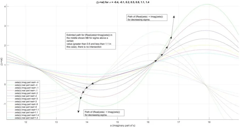
Figure 2. Riemann Zeta Function Detail Around a Known Zero

Focussing on the points where the real and imaginary parts intersect for various values of σ around a known zero of the zeta function in figure 2, we can see that the intersection points are at different values along an apparent single valued curve with an always positive derivative. This already gives an indication that it is very unlikely that there can be more than one zero along the curve depicting Re(ζ(s))=Im(ζ(s)) in the region of a specific value of a (ie that each value of a can have at most one zero of the eta function).

The next step is to follow a more formal approach to showing that that there can be not be more than one zero along the curve depicting the value of Re(ζ(s)) when (Re (ζ(s))=Im (ζ(s)) in the region of a specific value of a (ie that each value of a can have at most one zero of the zeta function).

III. METHODOLOGY - FORMAL

APPROACH TO DESCRIBING THE PATH OF THE FUNCTION DEPICTING THE

VALUE OF Re(ζ(s)) when

(Re(ζ(s))=Im(ζ(s))) IN THE

CRITICAL STRIP BY USING THE DIRICHLET ETA

FUNCTION.

For all that follows, we shall restrict the value of b between +1/2 to –1/2 (which means restricting σ between 0 and 1).

Riemann proved in his original paper that all zeros of the Riemann xi function have t with imaginary parts inside the region of +1

2i to -1

2i, which is equivalent to restricting b and σ. This means that the zeta function only has zeros in this region (the critical strip).

A. Zeta Function Zeros for 0<Σ<1.

In the well known Dirichlet η function (DLMF25.2.3) (also known as the alternating zeta function, which is continuous and continuously differentiable), which is related to the zeta function by η(s)=(1 − 21−𝑠_)ζ_{(s) and is} convergent (uniformly not absolutely) for σ>0, we have an expression that can be used to explore the characteristics of the real component, imaginary component and/or function zeros of the zeta function in the critical strip. It is important to note that (1 − 21−𝑠_{) does not have any zeros} for 0≤σ<1. It has an infinite number of zeros for σ=1.

It is important to emphasize that the relation between ζ(s) and η(s) shows that the two functions have the same zeros for 0<σ<1.

(4)

B. Eta Function Real and Imaginary Components for σ>0.

Investigating the real and imaginary components of η(s). Starting with:

η(s) = ∑ (−1)𝑛−1

𝑛𝑠 ∞

𝑛=1 = (1

-1 2𝑠+

1 3𝑠−

1 4𝑠 +...)

Extracting the real and imaginary parts for one term (remembering that s= (σ+ai)):

1 𝑛𝑠=

1

𝑛𝜎_{(cos(𝑎𝑙𝑜𝑔(𝑛))+𝑖𝑠𝑖𝑛(𝑎𝑙𝑜𝑔(𝑛)))}

= 𝑛𝜎 (cos(𝑎𝑙𝑜𝑔(𝑛))−𝑖𝑠𝑖𝑛(𝑎𝑙𝑜𝑔(𝑛))) (𝑛𝜎_{cos (𝑎𝑙𝑜𝑔(𝑛)))^2+(𝑛}𝜎_{sin(𝑎𝑙𝑜𝑔(𝑛)))^2}

= (cos(𝑎𝑙𝑜𝑔(𝑛))−𝑖𝑠𝑖𝑛(𝑎𝑙𝑜𝑔(𝑛))) 𝑛𝜎

This leads to the series representation of the real part as:

1 –cos (𝑎𝑙𝑜𝑔(2))

2𝜎 +

cos (𝑎𝑙𝑜𝑔(3))

3𝜎 −

cos (𝑎𝑙𝑜𝑔(4))

4𝜎 +... Exp 1

This leads to the series representation of the imaginary part as:

sin(𝑎𝑙𝑜𝑔(2))

2𝜎 −

3𝜎 +

sin (𝑎𝑙𝑜𝑔(4))

4𝜎 − ... Exp 2

C. Investigating Eta Function Real Component Equal to Imaginary Component and Value of the Real

Component.

Firstly equating the expressions for the real and imaginary components:

1 –cos (𝑎𝑙𝑜𝑔(2))

2𝜎 +

cos (𝑎𝑙𝑜𝑔(3)) 3𝜎 −... =

2𝜎 −

3𝜎 +

⋯

⇒1 –cos (𝑎𝑙𝑜𝑔(2))

2𝜎 +

cos (𝑎𝑙𝑜𝑔(3)) 3𝜎 −... –(

2𝜎 −

3𝜎 + ⋯ ) = 0 Exp 3

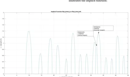
This gives an an implicit function which describes the values of σ and a when Re(η(s))=Im(η(s)). Figure 3 below illustrates the implicit function:

(5)

Note the separation of the points on the curve with horizontal and vertical tangents.

Totally differentiating Exp 3: log(2)cos(𝑎𝑙𝑜𝑔(2))

2𝜎 𝑑𝜎 𝑑𝑎+

log(2)sin(𝑎𝑙𝑜𝑔(2))

2𝜎 −

log(3)cos(𝑎𝑙𝑜𝑔(3)) 3𝜎

𝑑𝜎 𝑑𝑎−

3𝜎 + ⋯ +

log(2)sin(𝑎𝑙𝑜𝑔(2)) 2𝜎

𝑑𝜎 𝑑𝑎−

log(2)cos(𝑎𝑙𝑜𝑔(2))

2𝜎 −

log(3)sin(𝑎𝑙𝑜𝑔(3)) 3𝜎

𝑑𝜎 𝑑𝑎+

3𝜎 + ⋯ = 0

⇒𝑑𝜎_𝑑𝑎 = (−log(2)sin(𝑎𝑙𝑜𝑔(2))

2𝜎 +

3𝜎 +

2𝜎 −

3𝜎 + ⋯ )/(+

2𝜎 −

3𝜎 +

2𝜎 −

3𝜎 + ⋯ ) Exp 4

If we now totally differentiate Exp 1 and substitute in the 𝑑𝜎 𝑑𝑎 expression above (since we are investigating the real component value when the real component is equal to the imaginary component), we will have an expression that describes the derivative of the expression that describes the real component value when the real component equals the imaginary component:

Totally differentiating Exp 1:

D(Exp 1) = log(2)cos(𝑎𝑙𝑜𝑔(2)) 2𝜎

𝑑𝜎 𝑑𝑎 +

2𝜎 −

3𝜎 𝑑𝜎 𝑑𝑎−

3𝜎 + ⋯

⇒ D(Exp 1) = 𝑑𝜎 𝑑𝑎(

log (2)cos (𝑎𝑙𝑜𝑔(2))

2𝜎 −

log (3)cos (𝑎𝑙𝑜𝑔(3)) 3𝜎 +...) +log (2)sin(𝑎𝑙𝑜𝑔(2))

2𝜎 −

log (3)sin(𝑎𝑙𝑜𝑔(3))

3𝜎 + ⋯ Exp 5

Expressions 4 and 5 are convergent for σ>0 (from the uniform convergence of the eta function series, but can also be seen from the fact that log(𝑛)

𝑛𝜎 eventually becomes a monotonically reducing series tending to zero from a (large) value of n for any value of σ>0, which together with the Dirichlet test shows convergence).

The implicit function theorem (DLMF1.5) tells us that expression 4 (since expression 3 is continuously differentiable) describes a curve with neighbourhoods where σ is a function of a, except where 𝑑𝜎

𝑑𝑎 is undefined as the denominator is zero.

The same process can be used to show that: 𝑑𝑎

𝑑𝜎 = (−

2𝜎 +

3𝜎 −

2𝜎 +

3𝜎 + ⋯ )/(+

2𝜎 −

3𝜎 −

2𝜎 +

3𝜎 + ⋯ ) Exp 6 And:

D(Exp 1) = 𝑑𝑎 𝑑𝜎(

log (2)sin (𝑎𝑙𝑜𝑔(2))

2𝜎 −

log (3)sin (𝑎𝑙𝑜𝑔(3)) 3𝜎 +...) +log (2)cos(𝑎𝑙𝑜𝑔(2))

2𝜎 −

log (3)cos(𝑎𝑙𝑜𝑔(3))

3𝜎 + ⋯ Exp 7

It is important to note that expression 7 is equivalent to expression 5 (they describe the same function).

Similarly the implicit function theorem tells us that expression 6 describes a curve with neighbourhoods where a is a function of σ, except where 𝑑𝑎

𝑑𝜎 is undefined as the denominator is zero.

At this point it is useful to note the Harmonic Addition Theorem (Oo and Gan, 2010) and its implications for expressions 5 and 7 when expressions 4 and 6 are substituted in.

Restating the harmonic addition theorem:

Given 𝑥𝑠(𝑡) = ∑𝐿𝑖=1𝛼𝑖sin(𝜔0𝑡 + 𝜙𝑖) or

𝑥𝑐(𝑡) = ∑𝐿𝑖=1𝛼𝑖cos(𝜔0𝑡 + 𝜙𝑖), it is possible to find 𝛽 and 𝜓 so that 𝑥𝑠(𝑡) = 𝛽sin(𝜔0𝑡 + 𝜓) or 𝑥𝑐(𝑡) = 𝛽cos(𝜔0𝑡 + 𝜓), where:

𝛽 = (∑𝐿𝑖=1𝛼𝑖 2

+ 2 ∑ ∑𝐿𝑗=𝑖+1𝛼𝑖𝛼𝑗cos(𝜙𝑖− 𝜙𝑗)) 1 2 𝐿−1

𝑖=1 and:

Ψ = arg∑𝐿𝑖=1𝛼𝑖𝑠𝑖𝑛𝜙𝑖 ∑𝐿𝑖=1𝛼𝑖𝑐𝑜𝑠𝜙𝑖

, -π < 𝜓≤ π.

In the limit as L increases, the expression for 𝛽 does not appear to converge. For the next steps of the process, we shall consider partial sums of the Dirichlet eta function (ie n ranges from 2 to L (however large) and not necessarily to

∞.

With the above constraint, if we now use the harmonic addition theorem combined with expressions 5 and 4, substituting log(2) for 𝜔0 and a for t and noticing that the

(6)

𝑑𝜎 𝑑𝑎=(−

2𝜎 +

3𝜎 +

2𝜎 −

3𝜎 + ⋯ )/(+

2𝜎 −

3𝜎 +

2𝜎 −

3𝜎 + ⋯ )

⇒𝑑𝜎_𝑑𝑎 =(-𝛽 sin(log(2) 𝑎 + 𝜓) + 𝛽 cos(log(2) 𝑎 + 𝜓))/(𝛽 cos(log(2) 𝑎 +

𝜓) + 𝛽 sin(log(2) 𝑎 + 𝜓)) Exp 8

And: D(Exp 1)=

((-𝛽 sin(log(2) 𝑎 + 𝜓) + 𝛽 cos(log(2) 𝑎 + 𝜓))/(𝛽 cos(log(2) 𝑎 + 𝜓) +

𝛽 sin(log(2) 𝑎 + 𝜓)))*( 𝛽 cos(log(2) 𝑎 + 𝜓))+ 𝛽 sin(log(2) 𝑎 + 𝜓)

⇒ D(Exp 1)= 𝛽/(cos(log(2) 𝑎 + 𝜓) + sin(log(2) 𝑎 + 𝜓)) or:

D(Exp 1) = 𝛽 csc(log(2) 𝑎 + 𝜓 + 𝜋/4)/√2 Exp 9

Using the same approach with expressions 7 and 6: 𝑑𝑎

𝑑𝜎 =

(-𝛽 sin(log(2) 𝑎 + 𝜓) − 𝛽 cos(log(2) 𝑎 + 𝜓))/(−𝛽 cos(log(2) 𝑎 + 𝜓) +

𝛽 sin(log(2) 𝑎 + 𝜓)) Exp 10

And:

D(Exp 1) = −𝛽 csc(log(2) 𝑎 + 𝜓 − 𝜋/4)/√2 Exp 11

Note that expressions 9 and 11 are equivalent - they describe the same function.

Expressions 8-11 deserve close study.

Firstly, we can look at 𝛽 in more detail. Starting from the definition of 𝛽 above:

𝛽 = (∑𝐿𝑖=1𝛼𝑖 2

+ 2 ∑ ∑𝐿𝑗=𝑖+1𝛼𝑖𝛼𝑗cos(𝜙𝑖− 𝜙𝑗)) 1 2 𝐿−1

𝑖=1

Note that 𝛽 as an amplitude does not change sign for varying values of σ and a (given we that we do not rearrange any series), but potentially has a minimum of zero. It is also useful to note that in general, the limit as x→0 of yx/x is y and of y(x^2)/x is 0.

In fact, it seems that 𝛽 does not equal zero in any of the above expressions (although this is not a necessary result for the purposes of this paper). This is because for 𝛽 to be zero then in the expression 𝑥𝑐(𝑡) = ∑𝐿𝑖=1𝛼𝑖cos(𝜔0𝑡 + 𝜙𝑖), , 𝑥𝑐(𝑡) would be zero for all t (ie the expression would be identically zero for all t). This would mean that, given that 𝜙𝑖are all fixed, they would need to be zero or multiples of π (or appropriate multiples of expressions including π, such that the

∑𝐿𝑖=1𝛼𝑖cos(𝜔0𝑡 + 𝜙𝑖) summed identically to zero for any t). In the particular case here, where 𝜙𝑖 = (alog(n)-alog(2)), this is

not the case. This means that in this case, 𝛽≠ 0.

The csc function has no zeros (and is undefined in between sections of alternating all positive values and all negative values) . All expressions are valid for all σ and a values for the eta function (and describe a single valued function for each σ,a input) - except those points where 𝑑𝜎

𝑑𝑎

and 𝑑𝑎

𝑑𝜎are undefined.

More specifically, firstly looking at expressions 8 and 9: Expression 8 describes a number of curves with neighbourhoods where σ is a function of a, except where expression 8 is undefined when the denominator is zero. Expression 9 gives the derivative of the function which describes the value of the real part of η(s) in those neighbourhoods, which is positive(negative) in one neighbourhood where σ is a function of a (ie the value of the real part of η(s) increases(decreases) for increasing a), is undefined at the same points where expression 8 is undefined and is negative(positive) in the adjacent neighbourhood (ie the value of the real part of η(s) increases(decreases) for decreasing a). This means that each separate curve segment describing the value of the real part of η(s) when Re(η(s)) = Im(η(s)) always has a positive(negative) derivative.

The same argument holds for expressions 10 and 11 (except that a is now a function of σ) and Expression 11 gives the derivative of the function which describes the value of the real part of η(s) in those neighbourhoods, which is positive(negative) in one neighbourhood where a is a function of σ (ie the value of the real part of η(s) increases(decreases) for increasing σ), is undefined at the same points where expression 10 is undefined and is negative(positive) in the adjacent neighbourhood (ie the value of the real part of η(s) decreases(increases) for increasing σ. This means that each separate curve segment describing the value of the real part of η(s) when Re(η(s)) = Im(η(s)) always has a positive(negative) derivative.

It is important to note that expressions 8 and 10 are undefined at different values - which means that we can define the function completely (with no change of sign for the total derivative of the function) at all points since expressions 8 and 10 describe the same function.

(7)

or all negative derivatives (derivative does not change sign but might equal zero, although individual segments might have positive or negative derivatives) - which means that they can only have a single zero per curve. This, in turn, means that there can be only one zero in the local region of any particular value of a.

The result of this is that the function approximating the value of the real component of the eta function when the partial sums of the series representing the real and imaginary components of η(s) have the same value can have at most one zero for a discrete complete section of curve. This means that for any fixed value of a, η(s) can only have one zero (in order to have more zeros, then the derivative would need to change sign at some point). This, combined with the facts that 1) the eta function zeros are the same as the zeta function zeros and 2) The Riemann xi function shows that a zeta function zero at s means there is a corresponding zero at (1-s), means that s and (1-s) must have the same real component (1/2).

These results hold for any value of a and for any value of L. This means that even though the expression for 𝛽 does not at

first sight appear to converge, we could argue that the derivative will not change sign when L tends to the limit. More rigorously, we can argue that (based on the fact that partial sums of series approach the value of the series with a known estimate of the error as the number of terms in the partial sum increases) for any value of a we can show that the real component of the eta function has a single zero to any required degree of accuracy (by increasing L).

We can further note that in the expression for 𝜓 that is:

Ψ = arg∑𝐿𝑖=1𝛼𝑖𝑠𝑖𝑛𝜙𝑖 ∑𝐿𝑖=1𝛼𝑖𝑐𝑜𝑠𝜙𝑖

, -π < 𝜓≤ π.

The two series in the expression both converge (the 𝛼𝑖 terms are of alternating sign and strictly reducing in magnitude and both the sin and cos series are actually phase shifted versions of the cos(xlog(n)) and sin(xlog(n)) series - by xlog(2) - which have already been proved to be bounded for all partial sums) - which means that 1) in the limit the expression for Ψ

converges and 2) we can evaluate the value of 𝛽 by using the

value of Ψ and thee values of the convergent series for real and imaginary components. This in turn means that we can evaluate 𝛽 in the case of the infinite series without formally

proving the convergence of the series for 𝛽 (although I suspect

it may converge).

The implication is that the Riemann Hypothesis is true.

IV. CONCLUSIONS

Known previously - The Riemann zeta function does not have zeros outside the critical strip.

In Section 2 the apparent behaviour of the paths of the points where Re(ζ(s))=Im(ζ(s)) were observed, showing that it was unlikely that there would be 2 zeros of ζ(s) for the same value of a (the imaginary component of s). In addition, the property of the Riemann xi function that ξ(s) = ξ(1-s) was noted.

In section 3A the Dirichlet eta function was introduced as an appropriate mechanism for investigating the zeros of the zeta function for ζ(s) where σ>0.

In Section 3B the convergent series representation of the real and imaginary parts of the eta function were established.

In section 3C the convergent series representations of the derivative of the implicit function describing the function where the real part is equal to the imaginary part of the eta function was established. Combined with the series representations of the derivative of the real part of the function when the real part is equal to the imaginary part and using the harmonic addition theorem (and initially working with partial sums due to the apparent non-convergence of resulting expressions) it was shown that the derivative will not change sign along any specific curve (ie curves that have all positive derivatives or all negative derivatives). This is then extended to infinite series.

This leads to the conclusion that the real component of the eta function where the real part of eta equals the imaginary part of eta has only a single zero for a fixed value of a (the imaginary part of s), which can be shown to any required degree of accuracy by increasing L (the number of terms in the partial sum). It is also implied (by the non-converging expression) that the derivative does not change sign for any value of L, removing the need for relying on partial sums.

(8)

component (a) there is at most one root, which means that since ξ(σ+ai) = ξ(1-(σ+ai)) those roots will be at σ=1/2 - which means that the Riemann Hypothesis is true.

V. ACKNOWLEDGEMENT

This research was self-funded.

VI. REFERENCES

DLMF, https://dlmf.nist.gov/1.5 DLMF, https://dlmf.nist.gov/25.2.E3

Edwards, H.M. 2001, Riemann's Zeta Function, Dover

Publications, USA.

N. Oo, W.-S. Gan 2012, 'On harmonic addition theorem', International Journal of Computer and Communication Engineering, vol. 1, no. 3, pp. 200-202.

Riemann, B., 1892, Gesammelte Werke, Teubner,