Exchange Rate Volatillity and Exports of Malaysian Manufactured Goods to China: An Empirical Analysis

(1)

EXCHANGE RATE VOLATILITY AND EXPORTS OF

MALAYSIAN MANUFACTURED GOODS TO CHINA:

AN EMPIRICAL ANALYSIS

Hock-Tsen Wong♣ Universiti Malaysia Sabah

Hock-Ann Lee

Universiti Malaysia Sabah

♣ Corresponding author: Faculty of Business, Economics and Accountancy, Universiti Malaysia Sabah, Jalan UMS, 88400, Kota

Kinabalu, Malaysia. E-mail: htwong@ums.edu.my

International Journal of Business and Society, Vol. 17 No. 1, 2016, 145 - 159

ABSTRACT

The impact of exchange rate volatility on international trade is an important issue in international economics. This study investigates the impact of exchange rate volatility on disaggregated bilateral exports of Malaysian manufactured goods to China. Exchange rate volatility is estimated by the threshold generalized autoregressive conditional heteroscedasticity (TGARCH) model, more specifically the TGARCH(1,1) model. The Johansen cointegration method and the dynamic ordinary least squares (DOLS) estimator are used in the estimation. There is some evidence of exchange rate volatility to have significant impact on real exports. Moreover, the impact of exchange rate volatility on real export can be negative or positive. The exports competitiveness of Malaysia should be improved. Exports shall be further diversified with more focused on intra-regional trade in Association of Southeast Asian Nations Economic Community (AEC).

Keywords: Exchange Rate Volatility; Exports; Manufactured Goods; Malaysia; China.

1. INTRODUCTION

(2)

146

4.9 per cent of total exports of manufactured goods and exports of transport equipment were RM10,212 million or about 2 per cent of total exports of manufactured goods (MOF, 2013).

The composition of exports of Malaysia shifted from comprising mainly agriculture and mining products in the 1960s to manufactured goods in the 1980s. The development and growth of the manufacturing sector was rapid in the late 1990s (MOF, 2011). The manufactured goods are the largest component of total exports. The main exports of Malaysia are machinery and transport equipment. In 2012, exports of electronics, electrical and appliances were Malaysian ringgit (RM) RM231,225 million or about 44.6 percent of total exports of manufactured goods, exports of chemical, chemical and plastic products were RM52,140 million or about 10.0 percent of total exports of manufactured goods, exports of machinery and equipment were RM25,197 million or about 4.9 percent of total exports of manufactured goods and exports of transport equipment were RM10,212 million or about 2 percent of total exports of manufactured goods (MOF, 2013).

The impact of exchange rate volatility on international trade is an important issue in international economics (Bahmani-Oskooee and Hegerty, 2007; Fang, Lai and Miller, 2009; Ćorić and Pugh, 2010; Bahmani-Oskooee and Harvey, 2011; Verheyen, 2012; Bahmani-Oskooee, Harvey and Hegerty, 2013; Nishimura, and Hirayama, 2013; Thorbecke and Kato, 2013; Baek, 2013, Wong, 2014). The rationale of examining the impact of exchange rate volatility on international trade is that exchange rate volatility induces uncertainty into international transactions. This uncertainty decreases international trade and economic welfare. Exporters and importers face uncertainty of their costs and revenues because of exchange rate risk

might reduce international transactions (Hall et al., 2010: 1514; Bahmani-Oskooee, Harvey

and Hegerty, 2014). However, there is no general consensus on the impact of exchange rate volatility on international trade. This suggests that the impact of exchange rate volatility on international trade shall be tested based on case by case basis. Moreover, mostly the recent studies in the literature use disaggregated data, namely bilateral international trade at the industry level.

China has been achieving rapid economic growth since the opening up of its economy in 1978. The growth of its manufacturing exports is said to be the main drive of its rapid economic growth. Moreover, manufacturing exports from China are said to be alternative to other manufacturing exports in Asian countries. Eichengreen, Rhee and Tong (2007) report that exports of China have a positive impact on exports of high income countries in Asia, namely Japan, Singapore and South Korea and also have a positive impact on middle income countries in Asia, namely Malaysia and the Philippines. On the other hand, exports of China is found to have a negative impact on exports of low income countries in Asia, namely Bangladesh, Cambodia, Sri Lanka and Pakistan. Conversely, Greenaway, Mahabir and Milner (2008) find no evidence of exports of China to have a negative impact on low income countries in Asia, namely Bangladesh, Cambodia, India, Pakistan and Vietnam but exports of high income countries in Asia, namely Korea, Singapore and Japan are adversely affected. Athukorala (2009) shows exports of China to have different impacts on exports of countries in East Asia. The impacts are found to be larger for Indonesia, Thailand, Malaysia and the Philippines and smaller for Japan and South Korea. Fu, Kaplinsky and Zhang (2012) report that the price

(3)

147

competition effects of exports of China for high income countries and low income counties diminish after the late 1990s. Exports of China have evolved from low price competition to product diversification and quality upgrading. Wong, Eng and Habibullah (2014) find that economic growth of China contributes to increase in consumption and investment of countries in Asia. However, economic growth of China is said to be more beneficial to countries in Asia positioned at upper stream of value chain and to be more harmful to countries in Asia positioned at downstream of value chain. Generally, these studies examine the impact of exports of China on exports of other countries in Asia using aggregated data.

This study investigates the impact of exchange rate volatility on disaggregated bilateral exports of Malaysian manufactured goods to China using monthly data for the period from 2010 to 2013. Previously, the impact of exchange rate volatility on export mainly examined using relatively low frequency data, namely yearly or quarterly data and also mostly using aggregated data or at the industry level. The impact of exchange rate volatility on export could be different across industries. Also, the impact of exchange rate volatility on a specific group of exports can be assessed more specifically by using disaggregated data. Moreover, there is limited study on the impact of exchange rate volatility on disaggregated bilateral exports in many Malaysia. China is a big economy in the World. Trade of Malaysia with China is becoming more important. In 2012, exports of Malaysia to China was RM88,746 million or 12.6 per cent of total exports whilst imports from China was RM91,865 million or 15.1 per cent of total imports (MOF, 2013). In the same year, exports of Malaysian manufactured goods to China was RM61,563 million or 13.7 per cent of total manufactured goods export (MOF, 2013). Manufactured goods are the most important exports of goods in Malaysia. Exchange rate volatility is estimated by the threshold generalized autoregressive conditional heteroscedasticity (TGARCH) model, more specifically the TGARCH(1,1) model. The standard export demand model is used, which is estimated as exports are a function of exchange rate, foreign demand and exchange rate volatility. The Johansen cointegration method and the dynamic ordinary least squares (DOLS) estimator are used in the estimation.

2. LITERATURE REVIEW

There is a vast amount of studies on the impact of exchange rate volatility on international trade (Bahmani-Oskooee and Hegerty, 2007; Wong and Tang, 2008, 2011; Fang, Lai and Miller, 2009; Ćorić and Pugh, 2010; Bahmani-Oskooee and Harvey, 2011; Verheyen, 2012; Bahmani-Oskooee, Harvey and Hegerty, 2013; Nishimura, and Hirayama, 2013; Thorbecke and Kato, 2013; Baek, 2013; Bahmani-Oskooee, Harvey and Hegerty, 2014; Wong, 2014). The rationale of examining the impact of exchange rate volatility on international trade is that exchange rate volatility induces uncertainty into international transactions. This uncertainty

decreases international trade and economic welfare (Hall et al., 2010: 1514). Nonetheless,

the impact of exchange rate volatility on international trade is theoretically and empirically ambiguous. Bahmani-Oskooee, Harvey and Hegerty (2014) investigate the impact of exchange rate volatility on trade between the United States (US) and Spain for 131 US export industries and 88 import industries. The autoregressive distributed lag approach is used to estimate the model. The trade model is a reduced-form model, which trade flow is a function of the GDP of the importing country, the real Spanish against the US exchange rate and a measure of volatility. The data are disaggregated to SITC 3-digit level for the period from 1962 to 2009.

(4)

148

The results show that exchange rate volatility has significant short-run impacts in about half of the industries. The US exports seem to show more of a response to exchange rate volatility than do Spanish exports. The long-run impact of exchange rate volatility shows that of the 74 cointegrated US export industries, 11 have positive coefficients and 24 have negative coefficients. The rest are mostly not affected. This demonstrates the impact of exchange rate volatility is not uniformly. There is some evidence of smaller industries might be more likely to respond positively to exchange rate volatility. This proposes that specialised goods might increase with exchange rate volatility.

The impact of exchange rate volatility on international trade is found to be negative in the short run but the magnitude is relatively small compared with other explanatory variable such as income. Verheyen (2012) examines disaggregated exports of SITC 0 to 9 of the eleven countries of the European Monetary Union, namely Austria, Belgium, Spain, Finland, France, Germany, Greece, Ireland, Italy, the Netherlands and Portugal to the US. The data are monthly for the period from January, 1995 to August, 2010. The results show that exchange rate volatility is mostly found to have a negative impact on international trade but its impact is relatively small with the estimated long-run elasticities are mostly less than unity. The long-run elasticities of the real exchange rate or the US industrial production are mostly larger than unity. Exports of 6 and 7 are mostly affected by exchange rate volatility. It is difficult for a country in a union currency to avoid the impact of exchange rate volatility because the impact of exchange rate volatility is not the same across industries and countries in one exchange rate policy. Exchange rate volatility does not affect Dutch exports to the US. Italian exports are depressed in many cases. Irish exports benefit from exchange rate volatility.

The impact of exchange rate volatility is found to be asymmetric across industries and countries. Nishimura and Hirayama (2013) inspect the impact of the Reminbi against Japanese Yen exchange rate volatility on international trade between Japan and China. The data are daily for the period from January, 2002 to December, 2011. Two measures of exchange rate volatility are used, namely the Exponential Generalized ARCH (EGARCH) model. That is, the autoregressive(1)-EGARCH(1,1) model and the standard deviation. The results show that Japanese exports to China are not affected by exchange rate volatility but Chinese exports to Japan are affected by exchange rate volatility. The exchange rate level is found not to have a significant impact on Japanese exports but it has a significant impact on Chinese exports. This may due to differences in the depth and the development of financial markets in the two countries.

In a summary, there are many studies investigating the impact of exchange rate volatility on international trade. However, mostly the recent studies in the literature use disaggregated data, namely bilateral international trade at the industry level. This enables the impact of exchange rate volatility on export to be assessed more accurately. The impact of exchange rate volatility is mostly found to be negative but the magnitude is relatively small compared with the magnitude of other explanatory variable such as foreign demand. The impact of exchange rate volatility can be asymmetric across industries and countries. The impact of exchange rate volatility on international trade shall be examined based on case-by-case basis.

(5)

149

3. DATA AND METHODOLOGY

Real total export is the sum of export values of standard international trade code (SITC) 5, SITC 6, SITC 7 and SITC 8 divided by total export price index (2005 = 100), which is constructed by taking the weights of export price indexes of SITC 5, SITC 6, SITC 7 and SITC 8, respectively (2005 = 100). Real exports of SITC 5, SITC 6, SITC 7 and SITC 8 are export values of SITC 5, SITC 6, SITC 7 and SITC 8 divided by export price indexes of SITC 5, SITC 6, SITC 7 and SITC 8, respectively. SITC 5 is chemicals and related products. SITC 6 is manufactured goods classified by material. SITC 7 is machinery and transport equipment. SITC 8 is miscellaneous manufactured articles. In this study, SITC is based on SITC, revision 4 of the United Nations. Real exchange rate is the RM against renminbi (RMB) exchange rate multiplied by the ratio of consumer price index (CPI) of Malaysia (2005 = 100) over CPI of China (2005 = 100) (Bahmani-Oskooee and Hegerty, 2014). Exchange rate volatility is real exchange rate volatility estimated by the TGARCH(1,1) model. Real foreign demand is expressed by industrial value added of China (2005 = 100). Export values of SITC 5, SITC 6, SITC 7 and SITC 8 and their export price indexes, respectively are obtained from various

issues of Malaysia External Trade Statistics System, Department of Statistics Malaysia. The

RM against RMB exchange rate is obtained from the website of Bank Negara Malaysia. CPI of

Malaysia is obtained from Consumer Price Index, Department of Statistics Malaysia. CPI and

industrial value added of China are obtained from the website of National Bureau of Statistics of China. The sample period is from January, 2010 to December, 2013.

The threshold GARCH (TGARCH) model was proposed by Zakoian (1994) and Glosten, Jagannathan, and Runkle (1993). The TGARCH model defines the conditional variance as a linear piecewise function. More specifically, the TGARCH(1,1) is specified as follows:

(1)

ln !! =

�

+

�

ln !!!!+ !!

!!!= ! + ! !!!!! + !!!!! !!!!! + !"!!!!

!!!! = 1 if !!!!

! _{< 0}

0 if !_!!!! _{≥ 0}

where ln is logarithm, e is real exchange rate, u_t is a disturbance term, is the conditional

variance and D_(t-1) is an indicative variable. When is negative, the impact of on !!

!

!!!!! !!!!!

Bad news and good news are said to have different impacts on the conditional variance. Thus when δ ≠ 0 there is leverage effect and the impact of news is said to be asymmetric. The result of the TGARCH(1,1) Model is given in Table 1.

. When is non-negative, the impact of on is

!!! is (α + δ)!)!!!!! !!!!! !!!!! !!! !!!!!! .

Hock-Tsen Wong and Hock-Ann Lee

μ

+ γ

(6)

150

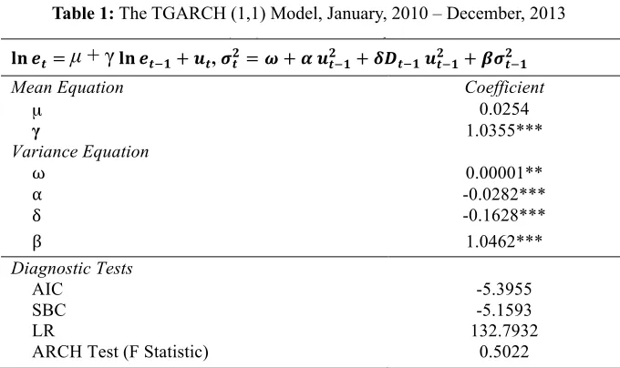
Table 1: The TGARCH (1,1) Model, January, 2010 – December, 2013

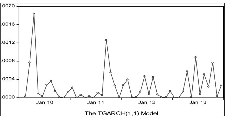
The coefficients of the mean equation and the variance equation are statistically significant, except the coefficient of the intercept of the mean equation. The coefficient of the leverage effect is found to be negative, less than one and statistically significant. Therefore there is asymmetric impact of the good news and the bad news on exchange rate volatility. One possible explanation of the leverage effect is that exporters are more worry about depreciation of RMB. The autoregressive conditional heteroskedasticity (ARCH) test (F statistic) for the disturbance term of the mean equation demonstrates that there is no ARCH effect and the estimated TGARCH(1,1) model is said to be appropriate. The plot of exchange rate volatility estimated by the TGARCH(1,1) model is given in Figure 1. Exchange rate volatility fluctuates over time. The mean and standard devaition of exchange rate volatility are 0.0003 and 0.0004, respectively. The Jarque-Bera test for exchange rate volatility is 136.1747, which is found to be statistically significant at 1 per cent level.

The standard export model to be estimated is specified as follows:

ln xt = β11 ln et + β12 ln yt + β13vt + u1,t (2)

where xt is real export (real total export, real export of SITC 5, real export of SITC 6, real export

of SITC 7 or real export of SITC 8), y_t is real foreign demand, v_t is exchange rate volatility,

which is estimated by the TGARCH(1,1) model and u1,t is a disturbance term. The export

model is usually estimated in logarithms, except the measure of exchange rate risk, which is in its level. The coefficient of real exchange rate is expected to be positive, which implies that an increase in real exchange rate or depreciation will lead to more exports. The coefficient of

Hock-Tsen Wong and Hock-Ann Lee 181

!!!= ! + ! !!!!! + !!!!! !!!!! + !"!!!!

!!!! = ! !" !!!!

! _!!

! !" !_!!!! _!! (1)

where ln is logarithm, e is real exchange rate, !! is a disturbance term, !!! is the

conditional variance and !!!! is an indicative variable. When !!!!! is negative, the

impact of !!!!! on !!! is (! + !)!!!!! . When !!!!! is non-negative, the impact of !!!!! on

!!! is !!!!!! . Bad news and good news are said to have different impacts on the

conditional variance. Thus when ! ≠ 0 there is leverage effect and the impact of news is

said to be asymmetric. The result of the TGARCH(1,1) Model is given in Table 1.

Table 1: The TGARCH (1,1) Model, January, 2010 – December, 2013

!" !!=�+� !" !!!!+ !!, !!!= ! + ! !!!!! + !!!!! !!!!! + !"!!!!

Mean Equation Coefficient

µ 0.0254

γ 1.0355***

Variance Equation

ω 0.00001**

α -0.0282***

δ -0.1628***

β 1.0462***

Diagnostic Tests

AIC -5.3955

SBC -5.1593

LR 132.7932

ARCH Test (F Statistic) 0.5022

Notes: et is real exchange rate. !! is a disturbance term. !!! is the conditional variance. !!!!

is an indicative variable. AIC is the Akaike information criterion. SBC is the Schwarz Bayesian criterion. LR is the log likelihood ratio. *** (**) denotes significance at the 1% (5%) level.

The coefficients of the mean equation and the variance equation are statistically significant, except the coefficient of the intercept of the mean equation. The coefficient of the leverage effect is found to be negative, less than one and statistically significant. Therefore there is asymmetric impact of the good news and the bad news on exchange rate volatility. One possible explanation of the leverage effect is that exporters are more worry about depreciation of RMB. The autoregressive conditional heteroskedasticity

Exchange Rate Volatility and Exports of Malaysian Manufactured Goods to China: An Empirical Analysis

(7)

151

Figure 1: Exchange Rate Volatility Estimated by the TGARCH(1,1) Model, January, 2010 – December, 2013

(3)

real foreign demand is expected to be positive if an increase in real foreign demand will lead to an increase in real export, which economic growth in manufacturing sector in China will encourage more exports of Malaysia. Conversely, the coefficient of real foreign demand is expected to be negative if economic growth in manufacturing sector in China will displace exports of Malaysia. The coefficient of exchange rate volatility is expected to be negative, which implies that exchange rate uncertainty will discourage exports of Malaysia.

Cointegration implies an error correction model, which can be expressed as follows:

182 Exchange Rate Volatility and Exports of Malaysian Manufactured Goods to China:

An Empirical Analysis

(ARCH) test (F statistic) for the disturbance term of the mean equation demonstrates that there is no ARCH effect and the estimated TGARCH(1,1) model is said to be appropriate. The plot of exchange rate volatility estimated by the TGARCH(1,1) model is given in Figure 1. Exchange rate volatility fluctuates over time. The mean and standard devaition of exchange rate volatility are 0.0003 and 0.0004, respectively. The Jarque-Bera test for exchange rate volatility is 136.1747, which is found to be statistically significant at 1 per cent level.

Figure 1: Exchange Rate Volatility Estimated by the TGARCH(1,1) Model, January, 2010 – December, 2013

.0000 .0004 .0008 .0012 .0016 .0020

Jan 10 Jan 11 Jan 12 Jan 13

The TGARCH(1,1) Model

The standard export model to be estimated is specified as follows:

ln !! = !!!ln !!+ !!"ln !!+ !!"!!+ !!,! (2)

where xt is real export (real total export, real export of SITC 5, real export of SITC 6,

real export of SITC 7 or real export of SITC 8), yt is real foreign demand, vt is exchange

rate volatility, which is estimated by the TGARCH(1,1) model and u1,t is a disturbance

term. The export model is usually estimated in logarithms, except the measure of exchange rate risk, which is in its level. The coefficient of real exchange rate is expected to be positive, which implies that an increase in real exchange rate or depreciation will lead to more exports. The coefficient of real foreign demand is expected to be positive if

where ec_t-1 is an error correction term generated from the Johansen cointegration method for

equation (2) and u_2,t is a disturbance term.

The DOLS estimator is also used to estimate real exports, which can be specified as follows:

(4)

where u_3,t is a disturbance term. The DOLS estimator corrects the problem of endogeneity by

including the leads (p) and lags (-p) of the first difference and the problem of serial correlation

by a generalized least squares procedure. The estimator provides good estimation in a finite sample (Stock and Watson, 1993).

(8)

152

4. RESULTS AND DISCUSSIONS

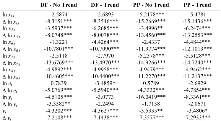
The results of the Dickey and Fuller and Phillips and Perron unit root test statistics are reported in Table 2. All the variables are mostly non-stationary in their levels but become stationary after taking the first differences, except real exports of SITC 5 and SITC 8, real foreign demand and exchange rate volatility. For real exports of SITC 5 and SITC 8 and real foreign demand, they could be the cases of border line or near to a unit root process. Thus, they are treated to be a unit root in this study. Exchange rate volatility will be entered as an exogenous variable in the long-run analysis since it is a stationary variable.

Table 2: The Results of the Dickey and Fuller (DF) and Phillips and Perron (PP) Unit Root Test Statistics

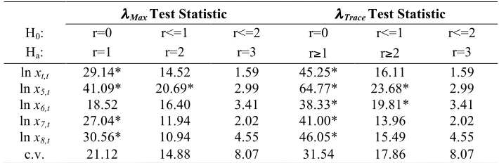
The results of the Johansen likelihood ratio test statistics, namely the maximum eigenvalue

statistic (λ_Max) and the trace statistic (λ_Trace) are computed with unrestricted intercepts and

no trends in the vector autoregressive model are reported in Table 3. The lag length used to compute the vector autoregressive model is based on the Schwarz Bayesian criterion (SBC). The results show that the null hypothesis of no cointegration among real export, real exchange rate and real foreign demand is rejected. As a result there is at least one cointegrating vector among those variables.

Table 2: The Results of the Dickey and Fuller (DF) and Phillips and Perron (PP) Unit Root Test Statistics

DF - No Trend DF - Trend PP - No Trend PP - Trend

ln xt,t -2.5874 -2.6893 -5.2178*** -5.4781

Δ ln xt,t -8.3151*** -8.3546*** -15.2669*** -15.1436***

ln x5,t -3.5937*** -6.2685*** -3.4996** -6.2474***

Δ ln x5,t -8.0748*** -8.0078*** -13.4560*** -13.2553***

ln x6,t -1.3221 -4.4264*** -2.4337 -4.4844***

Δ ln x6,t -10.7801*** -10.7090*** -11.9774*** -12.1013***

ln x7,t -2.5118 -2.7970 -5.2378*** -5.5128***

Δ ln x7,t -13.6769*** -13.4970*** -14.9266*** -14.7240***

ln x8,t -4.9892*** -4.9958*** -4.9479*** -4.9462***

Δ ln x8,t -10.4605*** -10.4400*** -11.2270*** -11.2137***

ln et 0.7839 -3.4859* 0.5789 -2.6929

Δ ln et -5.0769*** -5.5940*** -4.3332*** -4.7854***

ln yt -4.5105*** -3.0773 -16.0419*** -8.3361***

Δ ln yt -3.3382** -2.2494 -1.7138 -2.0671

vt -4.3202*** -4.3627*** -3.5335** -3.4806*

Δvt -7.2108*** -7.1438*** -7.3577*** -7.2933***

Notes: xt is real total export. xi,t is real export of SITC i (i = 5, 6, 7, 8). et is real exchange rate. yt is real

foreign demand. vt is exchange rate volatility estimated by the TGARCH(1,1) Model. DF - No Trend is

the Dickey and Fuller test statistic estimated with the model included a constant only. DF - Trend is the Dickey and Fuller test statistic estimated with the model included a constant and a time trend. PP - No Trend is the Phillips and Perron test statistic estimated with the model included a constant only. PP - Trend is the Phillips and Perron test statistic estimated with the model included a constant and a time trend. *** (**, *) denotes significance at the 1% (5%, 10%) level.

The results of the Johansen likelihood ratio test statistics, namely the maximum

eigenvalue statistic (λMax) and the trace statistic (λTrace) are computed with unrestricted

intercepts and no trends in the vector autoregressive model are reported in Table 3. The lag length used to compute the vector autoregressive model is based on the Schwarz Bayesian criterion (SBC). The results show that the null hypothesis of no cointegration among real export, real exchange rate and real foreign demand is rejected. As a result there is at least one cointegrating vector among those variables.

(9)

153

Table 3: The Results of the Johansen Likelihood Ratio Test Statistics

Table 3: The Results of the Johansen Likelihood Ratio Test Statistics

λMax Test Statistic λTrace Test Statistic

H0: r=0 r<=1 r<=2 r=0 r<=1 r<=2

Ha: r=1 r=2 r=3 r≥1 r≥2 r=3

ln xt,t 29.14* 14.52 1.59 45.25* 16.11 1.59

ln x5,t 41.09* 20.69* 2.99 64.77* 23.68* 2.99

ln x6,t 18.52 16.40 3.41 38.33* 19.81* 3.41

ln x7,t 27.04* 11.94 2.02 41.00* 13.96 2.02

ln x8,t 30.56* 10.94 4.55 46.05* 15.49 4.55

c.v. 21.12 14.88 8.07 31.54 17.86 8.07

Notes: xt is real total export. xi,t is real export of SITC i (i = 5, 6, 7, 8). c.v. is the 5% critical value. * denotes significance at the 5% level.

The results of the normalised cointegrating vectors are reported in Table 4. The likelihood ratio test statistics, which test that the coefficients of real exchange rate and real foreign demand are zero, respectively are mostly rejected. Generally, an increase in real exchange rate will lead to an increase in real export and an increase in real foreign demand will lead to a decrease in real export. On the whole, real exchange rate and real foreign demand are found to be important in the determination of real export.

Table 4: The Results of the Normalised Cointegrating Vectors

ln xt,t = 3.7008 ln et - 2.1161 ln yt (11.0063***) (12.7514***) ln x5,t = 2.5991 ln et - 0.5776 ln yt (19.6246***) (3.7283*) ln x6,t = 5.3958 ln et - 0.0430 ln yt (1.8789) (0.0088) ln x7,t = 8.8320 ln et - 6.6587 ln yt (8.7565***) (15.0966***) ln x8,t = 1.9806 ln et - 2.2524 ln yt (4.7273**) (17.4245***)

Notes: xt is real total export. xi,t is real export of SITC i (i = 5, 6, 7, 8). Values in parentheses are the likelihood ratio test statistics. *** (**, *) denotes significance at the 1% (5%, 10%) level.

This study uses the general to specific modelling strategy to find the error correction representation. Initially, three lags of each first difference variable are used and then the dimensions of the parameter space are reduced to a final parsimonious specification by sequentially excluding least statistically insignificant variables. The results of the error correction models (ECMs) are disclosed in Table 5. The plots of cumulative sum of

Table 3: The Results of the Johansen Likelihood Ratio Test Statistics

λMax Test Statistic λTrace Test Statistic

H0: r=0 r<=1 r<=2 r=0 r<=1 r<=2

Ha: r=1 r=2 r=3 r≥1 r≥2 r=3

ln xt,t 29.14* 14.52 1.59 45.25* 16.11 1.59

ln x5,t 41.09* 20.69* 2.99 64.77* 23.68* 2.99

ln x6,t 18.52 16.40 3.41 38.33* 19.81* 3.41

ln x7,t 27.04* 11.94 2.02 41.00* 13.96 2.02

ln x8,t 30.56* 10.94 4.55 46.05* 15.49 4.55

c.v. 21.12 14.88 8.07 31.54 17.86 8.07

Notes: xt is real total export. xi,t is real export of SITC i (i = 5, 6, 7, 8). c.v. is the 5% critical value. * denotes significance at the 5% level.

Table 4: The Results of the Normalised Cointegrating Vectors

ln xt,t = 3.7008 ln et - 2.1161 ln yt (11.0063***) (12.7514***) ln x5,t = 2.5991 ln et - 0.5776 ln yt (19.6246***) (3.7283*) ln x6,t = 5.3958 ln et - 0.0430 ln yt (1.8789) (0.0088) ln x7,t = 8.8320 ln et - 6.6587 ln yt (8.7565***) (15.0966***) ln x8,t = 1.9806 ln et - 2.2524 ln yt (4.7273**) (17.4245***)

Notes: xt is real total export. xi,t is real export of SITC i (i = 5, 6, 7, 8). Values in parentheses are the likelihood ratio test statistics. *** (**, *) denotes significance at the 1% (5%, 10%) level.

This study uses the general to specific modelling strategy to find the error correction representation. Initially, three lags of each first difference variable are used and then the dimensions of the parameter space are reduced to a final parsimonious specification by sequentially excluding least statistically insignificant variables. The results of the error correction models (ECMs) are disclosed in Table 5. The plots of cumulative sum of

Table 4: The Results of the Normalised Cointegrating Vectors

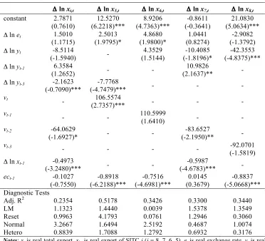
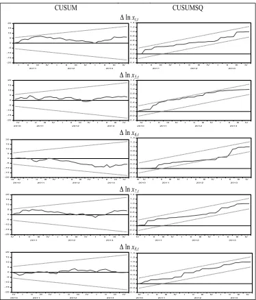
This study uses the general to specific modelling strategy to find the error correction representation. Initially, three lags of each first difference variable are used and then the dimensions of the parameter space are reduced to a final parsimonious specification by sequentially excluding least statistically insignificant variables. The results of the error correction models (ECMs) are disclosed in Table 5. The plots of cumulative sum of recursive residuals (CUSUM) and cumulative sum of squares of recursive residuals (CUSUMSQ) are reported in Figure 2. Generally, there is no evidence of instability of the ECMs. The estimations

(10)

154

Table 5: The Results of the Error-Correction Models

of the models are said to be appropriate. On the whole, the results show the ECMs to have a

high adjusted of the coefficient of determination (R2_{), that is, range from 0.2354 to 0.5178. The}

one period lags of error correction terms are majority found to be statistically significant. This implies that there is long-run relationship among the variables examined. The results show exchange rate volatility to have significant impact on real total export and real exports of SITC 5 and SITC 7. An increase in exchange rate volatility will lead to a decrease in real total export and real export of SITC 7 in the short run. Conversely, an increase in exchange rate volatility will lead to an increase in real export of SITC 5.

Exchange Rate Volatility and Exports of Malaysian Manufactured Goods to China: An Empirical Analysis

Table 5: The Results of the Error-Correction Models

Δ ln xt,t Δ ln x5,t Δ ln x6,t Δ ln x7,t Δ ln x8,t

constant 2.7871

(0.7610) (6.2218)*** 12.5270 (4.7363)*** 8.9206 (-0.3641) -0.8611 (5.0634)*** 21.0830 Δ ln et 1.5010

(1.1715) (1.9795)* 2.5013 (1.9800)* 4.8680 (0.8274) 1.0441 (-1.3792) -2.9082 Δ ln yt -8.5114

(-1.5940) - (1.5144) 4.3529 (-1.8196)* -10.4085 (-4.8375)*** -42.3553 Δ ln yt-1 6.3584

(1.2652) - - (2.1637)** 10.9826 -

Δ ln yt-3 -2.1623

(-0.7090)*** (-4.7479)*** -7.7768 - - -

vt _- 106.5574

(2.7357)*** - - -

vt-1 _- _- 110.5999

(1.6410) - -

vt-2 -64.0629

(-1.6927)* - - (-2.1950)** -83.6527 -

vt-3 _- _- _- _- -92.0701

(-1.5819) Δ ln xt-1 -0.4973

(-3.2480)*** - - (-4.6783)*** -0.5987 -

ect-1 -0.1027

(-0.7550) (-6.2188)*** -0.8918 (-4.6981)*** -0.7516 (0.3679) 0.0145 (-5.0668)*** -0.8837 Diagnostic Tests

Adj. R2 _0.2354 _0.5178 _0.3426 _0.3300 _0.3440

LM 1.1323 1.4440 0.0039 1.5378 1.3549

Reset 0.9963 4.1793 0.0761 1.2946 0.3060

Normal 3.2667 1.6494 2.5192 0.4687 1.0074

Hetero 0.8839 1.7088 1.2792 0.6932 0.3176

Notes: xt is real total export. xi,t is real export of SITC i (i = 8, 7, 6, 5). et is real exchange rate. yt is real foreign demand. vt is exchange rate volatility estimated by the TGARCH(1,1) Model. xj,t-1 is lag of real total export or real export of SITC i (i = 5 - 8). Adj. R2_{is the adjusted R}2_{. LM is the Lagrange Multiplier}

(11)

155

Figure 2: The Plots of Cumulative Sum of Recursive Residuals (CUSUM) and Cumulative Sum of Squares of Recursive Residuals (CUSUMSQ)

Note: xt is real total export. xi,t is real export of SITC i (i = 5, 6, 7, 8).

The results of the the DOLS estimator are presented in Table 6. The leads (p) and lags (

-p) of the first difference are selected based on the Akaike information criterion (AIC)

CUSUM CUSUMSQ

Δ ln xt,t

-20 -15 -10 -5 0 5 10 15 20

I II III IV I II III IV I II III IV 2011 2012 2013

-0.4 -0.2 0.0 0.2 0.4 0.6 0.8 1.0 1.2 1.4

I II III IV I II III IV I II III IV 2011 2012 2013

Δ ln x5,t

-20 -15 -10 -5 0 5 10 15 20

IV I II III IV I II III IV I II III IV 2010 2011 2012 2013

-0.4 -0.2 0.0 0.2 0.4 0.6 0.8 1.0 1.2 1.4

Δ ln x6,t

-20 -15 -10 -5 0 5 10 15 20

III IV I II III IV I II III IV I II III IV

2010 2011 2012 2013

-0.4 -0.2 0.0 0.2 0.4 0.6 0.8 1.0 1.2 1.4

III IV I II III IV I II III IV I II III IV

2010 2011 2012 2013

Δ ln x7,t

-20 -15 -10 -5 0 5 10 15 20

IV I II III IV I II III IV I II III IV 2011 2012 2013

-0.4 -0.2 0.0 0.2 0.4 0.6 0.8 1.0 1.2 1.4

IV I II III IV I II III IV I II III IV 2011 2012 2013

Δ ln x8,t

-20 -15 -10 -5 0 5 10 15 20

-0.4 -0.2 0.0 0.2 0.4 0.6 0.8 1.0 1.2 1.4

IV I II III IV I II III IV I II III IV

2010 2011 2012 2013

(12)

156

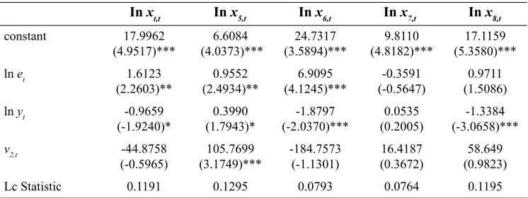
The results of the the DOLS estimator are presented in Table 6. The leads (p) and lags (-p) of the first difference are selected based on the Akaike information criterion (AIC) with the maximum lags are set for three. Exchange rate volatility is included in the estimation as a deterministic variable. The results of the Hansen parameter instability test, which is a test of the null hypothesis of cointegration against the alternative of no cointegration, are all not rejected at the 5 percent level. Thus all the estimated equations are stable in the long run. On the whole, there is no evidence of exchange rate volatility to have a significant impact of real total export but there is some evidence of exchange rate volatility to have a significant impact on disaggregated real export, that is, real export of SITC 5. The conclusion that exchange rate volatility to have a significant impact on disaggregated real export and not real total export is the same as the conclusion obtained by the Johansen method.

Table 6: The Long-Run Coefficients of the Dynamic Ordinary Least Squares (DOLS) Estimator

Notes: Lc statistic is the Hansen parameter instability test. The standard errors are the Newey-West standard errors. *** (**, *) denotes significance of the t-statistic at the 1% (5%, 10%) level.

In x_8,t In x_6,t In x_7,t

In x_5,t In x_t,t

constant 17.9962 6.6084 24.7317 9.8110 17.1159

(4.9517)*** (4.0373)*** (3.5894)*** (4.8182)*** (5.3580)***

ln et 1.6123 0.9552 6.9095 -0.3591 0.9711

(2.2603)** (2.4934)** (4.1245)*** (-0.5647) (1.5086)

ln yt -0.9659 0.3990 -1.8797 0.0535 -1.3384

(-1.9240)* (1.7943)* (-2.0370)*** (0.2005) (-3.0658)***

v2,t -44.8758 105.7699 -184.7573 16.4187 58.649

(-0.5965) (3.1749)*** (-1.1301) (0.3672) (0.9823)

Lc Statistic 0.1191 0.1295 0.0793 0.0764 0.1195

This study finds some evidence of the impact of exchange rate on exports of Malaysian manufactured goods to China, namely real total export and real exports of SITC 5 and SITC 7. However, there is no significant impact of exchange rate volatility on real exports of SITC 6 and SITC 8. The finding that exchange rate volatility to have significant impact on exports is consistent with the findings of Thorbecke and Kato (2013) and Bahmani-Oskooee, Harvey and Hegerty (2014), among others. A stable exchange rate is important to promote exports. An increase in exchange rate volatility would have negative or positive impact on some exports of Malaysian manufactured goods to China. Moreover, this study finds that real exchange rate and real foreign demand are mostly found to have significant impacts on real exports in the long run and short run. The coefficients of real exchange rate are mostly found to be positive whilst the coefficients of real foreign demand are mostly found to be negative. An increase in real exchange rate or depreciation of real exchange rate would lead to an increase in real export. An increase in real foreign demand will lead to a decrease in real export. This can be

(13)

157

some evidence of economic growth in China particularly in its manufacturing sector could have adverse impact on exports of Malaysian manufactured goods to China. The growth of manufacturing sector in China would replace some exports from Malaysia (Eichengreen, Rhee and Tong, 2007).

There is no strong evidence of exchange rate volatility on real export could be due to the exchange rate policy and its management implemented in Malaysia are satisfactory to avoid the adverse impact of exchange rate volatility on export. Malaysia adopts a managed floating exchange rate. In the long run, exporters of manufactured goods in Malaysia shall continue to improve their products through innovation and high technology. Technological improvement, innovation and knowledge driven activities in manufacturing sectors are crucial to remain competitive in exports. Innovation means breach into new markets, improve market share and increase returns. Innovation would lead to higher returns to workers. The pivotal is to expand innovation capabilities and to create continuous innovation. Disruptive innovations create new markets, which will replace existing markets and displace earlier technologies. Both continuous and disruptive innovations are important to increase productivity and move up the value chain to sustain economic growth in the long run (MOF, 2013). An effective marketing approach shall be adopted to promote exports of Malaysia. Exports shall be further diversified with more focused on intra-regional trade in Association of Southeast Asian Nations Economic Community (AEC), which was launched in 2010 with the aims to promote free flow of goods, services, investment, capital and skilled labour to attract investment and trade in the region. AEC would provide export market as well as challenge to exports of Malaysian manufactured goods in the region. The AEC region has a large population and its GDP per capita is increasing. The successful of AEC will support the national transformation programme of Malaysia is to foster its agenda to be a high income nation by 2020 (MOF, 2013).

5. CONCLUDING REMARKS

This study has investigated the impact of exchange rate volatility on real total export and real exports of SITC 8, SITC 7, SITC 6 and SITC 5. There is long-run relationship among real export, real exchange rate and real foreign demand. There is some evidence of exchange rate volatility to have significant impact on real exports. The impact of exchange rate volatility on real export can be negative or positive. An increase in real exchange rate or depreciation of real exchange rate will lead to more exports. An increase in real foreign demand will lead to a decrease in real export. The growth of manufacturing sector in China would replace some exports from Malaysia. In the long run, exporters of Malaysia shall improve their products through innovation and high technology. The exports competitiveness of Malaysia could be improved. Also, an effective marketing approach shall be used to further promote exports of Malaysia. Exports shall be further diversified with more focused on intra-regional trade in AEC, which would provide a good market opportunity for exports of Malaysian manufactured goods. The more diversified of export market would result more stable of economy of Malaysia. Exports can improve economic growth and can help Malaysia to transform its economy and to achieve its vision to be a high income country in the near future. Exports sector creates many employment opportunities. This can help to reduce the problem of unemployment in Malaysia.

(14)

158

ACKNOWLEDGEMENTS

The authors would like to thank Universiti Malaysia Sabah (UMS) for providing the funding of this study through UMS Research Grant Scheme (SBK0148-SS-2014). A version of the paper has been presented at and published in the proceedings of the International Borneo

Business Conference, Riverside Majistic Hotel, Kuching, Sarawak, Malaysia, 20th _{- 21}st

August 2014. The authors would like to thank the feedbacks from the participants of the International Borneo Business Conference 2014 and the useful comments from the reviewers of International Journal of Business and Society. All the remaining errors are the authors.

REFERENCES

Athukorala, P. C. (2009). The rise of China and East Asian export performance: Is the

crowding-out fear warranted? The World Economy, 32(2), 234-266.

Baek, J. (2013). Does the exchange rate matter to bilateral trade between Korea and Japan?

Evidence from commodity trade data. Economic Modelling, 30, 856-862.

Bahmani-Oskooee, M., & Harvey, H. (2011). Exchange-rate volatility and industry trade

between the U.S. and Malaysia. Research in International Business and Finance, 25(2),

127-155.

Bahmani-Oskooee, M., & Hegerty, S. W. (2007). Exchange rate volatility and trade flows: A

review article. Journal of Economic Studies, 34(3), 211-255.

Bahmani-Oskooee, M., Harvey, H., & Hegerty, S. W. (2013). The effects of exchange-rate

volatility on commodity trade between the U.S. and Brazil. The North American Journal

of Economics and Finance, 25, 70-93.

Bahmani-Oskooee, M., Harvey, H., & Hegerty, S. W. (2014). Exchange rate volatility and

Spanish-American commodity trade flows. Economic Systems, 38(2), 243-260.

Ćorić, B., & Pugh, G. (2010). The effects of exchange rate variability on international trade: A

meta-regression analysis. Applied Economics, 42(20), 2631-2644.

Eichengreen, B., Rhee, Y., & Tong, H. (2007). China and the exports of other Asian countries.

Review of World Economics, 143(2), 201-226.

Fang, W. S., Lai, Y., & Miller, S. M. (2009). Does exchange rate risk affect exports

asymmetrically? Asian evidence. Journal of International Money and Finance, 28(2),

215-239.

Fu, X., Kaplinsky, R., & Zhang, J. (2012). The impact of China on low and middle income

countries’ export prices in industrial-country markets. World Development, 40(8),

1483-1496.

(15)

159

Glosten, L. R., Jagannathan, R., & Runkle, D. E. (1993). On the relation between the expected

value and the volatility of the nominal excess return on stocks. Journal of Finance, 48(5),

1779-1801.

Greenaway, D., Mahabir, A., & Milner, C. (2008). Has China displaced other Asian countries'

exports? China Economic Review, 19(2), 152-169.

Hall, S., Hondroyiannis, G., Swamy, P. A. V. B., Tavlas, G., & Ulan, M. (2010). Exchange-rate volatility and export performance: Do emerging market economies resemble industrial

countries or other developing countries? Economic Modelling, 27(6), 1514-1521.

Ministry of Finance Malaysia (MOF). (2011). Economic Report 2011/2012. Kuala Lumpur,

Malaysia: Percetakan National Malaysia Berhad.

Ministry of Finance Malaysia (MOF). (2013). Economic Report 2013/2014. Kuala Lumpur,

Malaysia: Percetakan National Malaysia Berhad.

Nishimura, Y., & Hirayama, K. (2013). Does exchange rate volatility deter Japan-China

trade? Evidence from pre- and post-exchange rate reform in China. Japan and the World

Economy, 25-26, 90-101.

Stock, J., & Watson, M. (1993). A simple estimator of cointegrating vectors in higher order

integrated systems. Econometrica, 61(4), 783-820.

Thorbecke, W., & Kato, A. (2013). The effect of exchange rate changes on Japanese

consumption exports. Japan and the World Economy, 24(1), 64-71.

Verheyen, F. (2012). Bilateral exports from euro zone countries to the US - Does exchange rate

variability play a role? International Review of Economics & Finance, 24, 97-108.

Wong, C. Y., Eng, Y. K., & Habibullah, M. S. (2014). Rising China, anxious Asia? A Bayesian

new Keynesian view. China Economic Review, 28, 90-106.

Wong, H. T. (2014). Exchange rate volatility and international trade. Journal of Stock & Forex

Trading, 3(2), 1-3.

Wong, K. N., & Tang, T. C. (2008). The effects of exchange rate variability on Malaysia’s

disaggregated electrical exports. Journal of Economic Studies, 35(2), 154-169.

Wong, K. N., & Tang, T. C. (2011). Exchange rate variability and the export demand for

Malaysia’s semiconductors: An empirical study. Applied Economics, 43(6), 695-706.

Zakoian, J. M. (1994). Threshold heteroskedastic models. Journal of Economic Dynamics and

Control, 18(5), 931-955.