A Comparative Study on Sensitivity of Multivariate Tests of Normality to Outliers

(1)

A Comparative Study on Sensitivity of

Multivariate Tests of Normality to Outliers

Alao, Abiodun Nurudeen1*_{, Ayinde, Kayode}2_{, Solomon, Gbenga Sunday}3

1_{Department of Statistics, Kwara State Polytechnic, Ilorin, Nigeria} 2_{Department of Statistics, Federal University of Technology, Akure, Nigeria} 3_{Department of Statistics, Ladoke Akintola University of Technology, Ogbomoso, Nigeria}

Outliers are observations that are different from other observations in a data set. Their presence in Multivariate parametric statistical data analyses is rarely checked and this may lead to invalid inferences and misinterpretation of results. Multivariate tests of normality include Skewness (S), Kurtosis (K), Mardia Skewness (MS), Mardia Skewness for small sample (MSS), Mardia Kurtosis (MK), Shapiro-Wilk (SW), Shapiro-Francia (SF), Royston (R), Henze-Zirkler (HZ), Doornik-Harsen (DH), Energy (E), Gel-Gastwirth (GG), Bontemps-Meddahi (BM) and Desgagne-Micheaux (DM) tests. This research aims at identifying the multivariate normality tests that are more sensitive to outliers so as to avoid the menace it could cause in inferences. Monte Carlo experiments using R-programming code were conducted one thousands (1000) times by generating Multivariate normal data, at four (4) levels of dimension (p=2,3,4 and 5). Seven (7) sample sizes of (n = 10,20,30,50,100,120 and 150), and two (2) levels of percentage of generated data, k (10% and 20%) polluted with outliers t, at ten (10) various magnitudes. The sample sizes were classified into small (n=10 and 20), medium (n=30 and 50), and large (n=100,120 and 150). The power rate of the multivariate tests were examined and compared at three (3) levels of significance namely; 1%, 5% and 10%. At a particular classified sample size, a test is considered most sensitive if it has power rate closet to unity. The study revealed that the GG and DH multivariate tests were generally very sensitive to outliers. Furthermore, for large sample sizes, all the test statistics considered were very sensitive to the departure from normality as a result of outliers. In conclusion, the study recommends the use GG and DH for use in statistical inferences to avoid misleading interpretation of results.

Keywords: multivariate; outliers; sensitivity; normality tests

I. INTRODUCTION

Outliers are observations that are different from other observations. They are observations that lie outside the overall pattern of a distribution. They are generally data points that are far outside the norm for a variable or population (Jarrell,1994; Rasmussen,1988;Stevens,1984). Hawkins (1980,1981)

described an outlier as an observation that “deviates so much

from other observations as to arouse suspicions that it was generated by a different mechanism”. Outliers have also been defined as values that are “dubious in theeyes of the researcher”

(Dixon,1950) and contaminants (Wainer,1976). Outliers can have deleterious effects on statistical analyses because they generally serve to increase error variance and reduce the power

(2)

II. LITERATURE REVIEW

A careful review of the literature revealed that some work has been done to compare multivariate tests of normality. Mecklin and Mundford (2003) investigated the following eight tests of multivariate normality that used asymptotic critical values:

Mardia’s test for multivariate skewness, Mardia’s test of

multivariate kurtosis, the Mardia-Foster C2_{w omnibus}

statistic, the Mardia-Kent omnibus statistic, the Royston’s

multivariate Shapiro-Wilk test, the Romeu-Ozturk test, the Mudholkar-Srivasta-Lin extension of the Shapiro-Wilk test and the Henze-Zirkler empirical characteristic function test (Szekely & Rizzo, 2005). The authors evaluated the power of the eight tests in a Monte Carlo study against both the multivariate normal distribution and some alternatives to normality. A wide range of sample size and dimensions were used. They discovered that the tests of Foster, Mardia-Kent, Romeu-Ozturk and Mudholkar-Srivasta-Lin had Type 1 error rates in some of the situations exceed 0.10 (twice the normal rate of a=0.05) against data generated to be multivariate normal. They therefore concluded that no single test out of the compared statistics was found to be the most powerful. Ward (1988) compared the power of Merdia’s

skewness and kurtosis tests, the Malkovich-Afifi extension of the Shapiro-Wilk test, Hawkins extension of the Anderson- Darling test, the Mardia-Foster omnibus test and two of his own proposals that extended the Kolmogorov-Smirnov and Anderson-Darling tests. He concluded that Mardia’s Skewness

test, Hawkins tests and his own Anderson-Darling type test were the strongest. None of these tests, however, was good enough when tested against the multivariate distribution, which is a mild deviation from normality. He further noticed that the power of the Malkovich-Afifi test statistics, contrary to previous findings, decreased as the number of variables increased (Mardia ,1980a). Ward (1988) formulated a hypothesis that the power of these procedures seemed to be related to the correlation structure of the variance-covariance

matrix probably through their determinant. Although Mardia’s

tests seemed to be more effective, none of these was considered the best. Horsewell and Looney (1992) suggested that neither affine-invariant nor coordinate- dependent tests can be regarded as superior to others. They questioned the

‘diagnostic’ capabilities of this category of tests particularly

effective against the skewed or kurtotic alternatives. However, they stated that the performance of the skewness tests depend not only on the skewness of the distribution but also on the kurtosis. The power of skewness tests tend to be inflated when

compared to alternatives with greater than normal kurtosis and decreased when compared to alternatives with less than normal kurtosis. Richardson and Smith (1993) considered testing multivariate normality, focusing on the case of when the data are cross-sectionally correlated and also discussed how serial correlation can be accommodated. Their test is based on the over identifying restrictions from matching the first four moments of the data with those implied by the normal distribution. Czeslaw (2009) emphasized that a few comprehensive power studies for multivariate normality exist but none of them is fully comprehensive. He further added that majority of the most comprehensive studies have deliberately limited the scope of their work to a particular category of tests or to considering the most popular or promising tests. Solomon (2016) compare the Type I error rate and power of some multivariate normality tests at various levels of significance under different sample sizes and dimensions of multivariate data. He concluded that Type 1 error rate of HZ, MS, MSS, R and E are reasonably good while R, DH, GG, BM, and DM are affected by correlation.

III. MATERIALS AND

METHOD

In this study, Monte Carlo simulation studies were used to evaluate the sensitivity of the following multivariate normality tests of normality to outliers. The program for their evaluation was written using R package 3.1.1.

Let X1, X2, . . ., Xp be independent N-dimensional random

vector of an identical distribution defined by a distribution function Fp (X) as:

𝑋 =

[

𝑥

11

𝑥

12

⋯ 𝑥

1𝑝

𝑥

21

𝑥

22

⋯ 𝑥

2𝑝

⋮

⋮ ⋯ ⋮

𝑥

𝑁1

𝑥

𝑁2

⋯ 𝑥

𝑁𝑝]

=

[

𝑋

1'

𝑋

2'

⋮

𝑋

𝑁'

]

(1)

( )

~

P

,

X

N





where 𝜇 and∑are p-dimensional vectors

(3)

ASM Science Journal, Volume 12, Special Issue 5, 2019 for ICoAIMS2019

normality are: Replication(R) = 1000, Dimension (p) of

multivariate data =

2 ,

3 ,

4 and

5

, Percentage of Outlier (k) =

%

20 %

10 and

, Magnitude of Outlier (t) =

}

10 ,

,

3 ,

2 ,

1 {





t

, Sample size (Small, n=10,20; Medium, n=

30, 50; and Large, n= 100, 120 and 150); and level of

significance (



=

1 %,

5 %

and

10 %

).

The Monte Carlo experiments were conducted following these procedures. First, select the value of dimension (p) and sample size (n) for the experiment, then generate multivariate normally distributed sample using the equation of Ayinde and Adegboye[1] with the chosen dimensions and sample sizes. Then, randomly select k% of the generated multivariate normally distributed sample data generated using equal

probability selection method (EPSM). ij

y

replace the selected

observations with outlier contaminated data using the formula below:

p

j

n

i

y

Y

t

y

ij

max(

)

ij

;

1 ,

2 ,

,

;

1 ,

2 ,

,

*



=

+



=

(2)

Where

y

_ij*is the new observation as a result of outlier,

y

_ijis

the observation selected to be polluted with the outlier,

)

max(

Y

is the maximum of the observations in the vector of

data

Y

,and

t

is the Magnitude of outlier.Subject the multivariate tests of normality to the outlier polluted multivariate data and document the probability value

(

p

−

value

) associated with each test. Repeat the process all over for the number of replications (R).

Let

R

i

value

p

if

value

p

if

i

1 ,

2 ,

,

1 ,

0 

=











−



−

=





(3)

Estimate the power rate (the number of times the null hypothesis of normality is rejected) by

R

R i i



=

1





(4)

Then, repeat the process for different sample sizes and choose another dimension (

p

) and repeat the process until all other sample sizes, magnitudes of outlier and percentage of outlier are exhausted. The most sensitivity test statistics was identified

as follows: At a particular level of significance, the following steps are followed, count the number of times power rates are at least 0.9 over the level of Magnitude of outliers. Further count the number of times power rates are at least 0.9 over the percentage of outliers. Then, count the number of times power rates are at least 0.9 over the level of dimensions. The higher the number of counts the more sensitive the test is. Also, count again the number of times power rate are at least 0.9 over the classified sample sizes.

Therefore,

Sensitivity Rate at a particular sample size =𝑎⁄_𝐴 (5)

Where a = Total number of times in which power rates are at least 0.9 when counted over levels of dimensions, % of outliers, magnitude of outliers and classified sample sizes. A = product of the number of dimensions, levels of percentage (%) of outliers, levels of magnitudes and classified sample sizes.Thus,

Asmall= p * k* t* n (4 * 2*10* 2 =160);

Amedium= p*k* t* n ( 4 *2*10*2 =160);

ALarge = p* k* t* n( 4* 2* 10* 3 = 240) .

The closer the sensitivity rate is to 1, the more sensitive the test is to outliers.

IV. RESULT AND

DISCUSSION

The results of the sensitivity rates of the multivariate tests of normality at various levels of dimension, sample size, magnitude of outliers, and percentage of outliers are presented and discussed in this section at three levels of significance are presented in Table 1-3.

1. Results of Sensitivity Rate of Multivariate Tests of Normality to Outliers at 0.01 level

of significance

From Table 1, for small sample size categories, when n=10,

it can be observed that the order of sensitivity of the test is

MS=MK=MSS=S=K < HZ < E < DM < BM < SW < R < SF

<DH<GG and for n=20, the order of sensitivity is

(4)

G. Furthermore from Table 1, it can be observed that GG, DH

and R display higher sensitivity rate as compared to others

while MS, S, MK and K display low sensitivity rate for grouped

small sample. While for the medium sample sizes categories, it

can be observed that the order of sensitivity of the test is MK =

K < S= DM < SW <HZ=MS=MSS=R=DH=E=BM=SF=GG,

when the sample size is 30, and when the sample size is 50, the

order of sensitivity is MK=K < DM < HZ = MS =MSS = S =

SW=SF= E= R= DH=BM=GG. In Table1, K, MK and DM

display low sensitivity rate in that order as compared to others

while the rest display high sensitivity rate for grouped medium

sample.

For a large sample size categories, it can be observed that the

order of sensitivity of the test is

K<MK<HZ=MS=MSS=S=SF=SW=DM=E=R=BM=DH=GG

when n=100, when the sample size is 120 and 150 the order of

sensitivity are the same and in this order K= MK=

HZ=MS=MSS=S=SF=SW=DM=E=R=BM=DH=GG. Table 1

also shows that all test statistics display high sensitivity rate

for grouped large sample.

From Table 2, when the sample size is small, it can be

observed that the order of sensitivity of the test is

MS=MK=S=K< MSS <HZ<DM<E<R<SW=SF=BM<

DH=GG for n=10 and for n=20, it is

K<MK<DM<MS<S<SW<MSS<HZ=BM=SF=E=R=DH=G

G.

From Table 2, GG, DH, BM, SF,SW and R display higher

sensitivity rate as compared to others while S, MS, MK and

K display low sensitivity rate for grouped small sample. For

the medium sample sizes, it can be observed that the order

of sensitivity of the test for n = 30 is

K<MK<DM<HZ=SW=S=MS=MSS=R=E=BM=SF=GH=G

G while when the sample size is 50, the order of sensitivity

is

K=K<DM<HZ=MS=MSS=S=SW=SF=E=R=DH=BM=GG.

From Figure 5, all the test statistics display very high Table 1. Summary of Counts and Sensitivity Rates at 0.01 level of significance

Sample Size Classification/ Sensitivity Rate

Multivariate Normality Tests

HZ MS MK MSS R DH S K SW SF E GG BM DM

Small

10 4 0 0 0 70 77 0 0 68 71 40 78 66 62

20 78 75 28 78 80 80 71 20 78 78 78 80 79 66

Total 82 75 28 78 150 157 71 20 146 149 118 158 145 128

Exp.

count 160 160 160 160 160 160 160 160 160 160 160 160 160 160 Sensitivity 0.51 0.47 .0.18 0.49 0.94 0.98 0.44 0.13 0.91 0.93 0.74 0.99 0.91 0.8

Medium

30 80 80 66 80 80 80 78 66 79 80 80 80 80 78

50 80 80 70 80 80 80 80 70 80 80 80 80 80 74

Total 160 160 136 160 160 160 158 136 159 160 160 160 160 152 Exp.

count 160 160 160 160 160 160 160 160 160 160 160 160 160 160

Sensitivity 1 1 0.85 1 1 1 0.99 0.85 0.99 1 1 1 1 0.95

Large

100 80 80 79 80 80 80 80 76 80 80 80 80 80 80

120 80 80 80 80 80 80 80 80 80 80 80 80 80 80

150 80 80 80 80 80 80 80 80 80 80 80 80 80 80

Total 240 240 239 240 240 240 240 236 240 240 240 240 240 240 Exp.

count 240 240 240 240 240 240 240 240 240 240 240 240 240 240

(5)

sensitivity rate for grouped medium sample, although MK and

K are not as strong the rest.

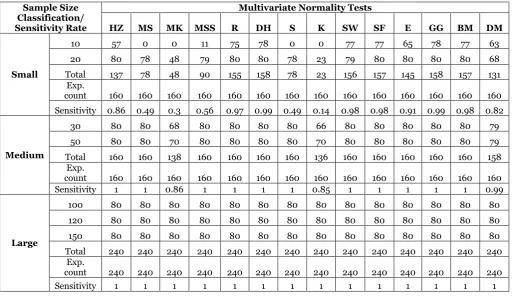
2. Results of Sensitivity Rate of Multivariate Tests of Normality to Outliers at 0.05 level of

significance

When the sample size is large, it can be observed that the order of sensitivity of the test is K = MK= HZ=MS=MSS=S=SF=SW=DM=E=R=BM=DH=GG for n=100, when n=120, it is

K=MK=HZ=MS=MSS=S=SF=SW=DM=E=R=BM=DH=GG, and when n=150, it is

K=MK=HZ=MS=MSS=S=SF=SW=DM=E=R=BM=DH=GG. Also, Table 2 reveals that all the test statistics display high sensitivity rate for grouped large sample.

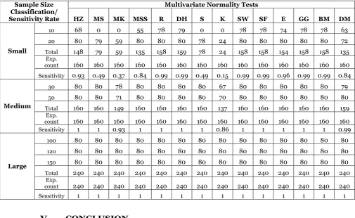
From Table 3, when the sample size is 10, the order of sensitivity of the test is

MS=MK=S=K< MSS <DM<HZ<E<SW=SF=R=BM=GG< DH and when the sample size is 20, it is

K<MK<DM<S<MS<HZ=MSS=SW=BM=SF=E=R=DH=GG. From Figure 3, GG, DH, BM, SF,SW and R display very high sensitivity rate as compared to others while S, MS, MK and K

display low sensitivity rate in that order for grouped small sample.

3. Results of Sensitivity Rate of Multivariate Tests of Normality to Outliers at 0.1 level of

significance

When the sample size is 30, the order of sensitivity of the

test is K<MK< DM

<HZ=SW=S=MS=MSS=R=E=BM=SF=GH=GG and for sample size n= 50, the order of sensitivity is K<MK < DM= HZ = MS =MSS = S = SW=SF= E= R= DH=BM=GG.

In Table 3, all the test statistics display near perfect sensitivity rate except MK and K for grouped medium sample.

When the sample size is large, it can be observed that the order of sensitivity of the test is

K=MK=HZ=MS=MSS=S=SF=SW=DM=E=R=BM=DH=G G for n=100, the order of sensitivity for n=120 is K= MK= HZ=MS=MSS=S=SF=SW=DM=E=R=BM=DH=GG and the order of sensitivity when n=150 is

Table 2. Summary of Count and Sensitivity Rate at 0.05 level of significance

HZ MS MK MSS R DH S K SW SF E GG BM DM

Small

10 57 0 0 11 75 78 0 0 77 77 65 78 77 63

20 80 78 48 79 80 80 78 23 79 80 80 80 80 68

Total 137 78 48 90 155 158 78 23 156 157 145 158 157 131

Exp.

count 160 160 160 160 160 160 160 160 160 160 160 160 160 160 Sensitivity 0.86 0.49 0.3 0.56 0.97 0.99 0.49 0.14 0.98 0.98 0.91 0.99 0.98 0.82

Medium

30 80 80 68 80 80 80 80 66 80 80 80 80 80 79

50 80 80 70 80 80 80 80 70 80 80 80 80 80 79

Total 160 160 138 160 160 160 160 136 160 160 160 160 160 158 Exp.

count 160 160 160 160 160 160 160 160 160 160 160 160 160 160

Sensitivity 1 1 0.86 1 1 1 1 0.85 1 1 1 1 1 0.99

Large

100 80 80 80 80 80 80 80 80 80 80 80 80 80 80

120 80 80 80 80 80 80 80 80 80 80 80 80 80 80

150 80 80 80 80 80 80 80 80 80 80 80 80 80 80

Total 240 240 240 240 240 240 240 240 240 240 240 240 240 240 Exp.

count 240 240 240 240 240 240 240 240 240 240 240 240 240 240

(6)

K=MK=HZ=MS=MSS=S=SF=SW=DM=E=R=BM=DH=GG. Also, in Table 3, all the test statistics display perfect sensitivity rate for grouped large sample.

V. CONCLUSION

In conclusions, it was generally observed that as sample size, percentage of outliers in the data set and magnitude of outliers increases, the sensitivity rate of the multivariate tests of normality depart from multivariate normality as a result of outlier in the data set. The multivariate tests in this order – GG, DH,R, BM, SF, HZ, E, SW, DM, MSS, MS, S, MK, K, are highly sensitive to departure from multivariate normality caused by outlier in the data set. Therefore, GG and DH tests can be considered to be the most sensitive to outliers in multivariate data set.

VI. ACKNOWLEDGEMENT

The first author wishes to record his gratitude and thanks to TETFUND, Nigeria, for the financial assistance.

Table 3. Summary of Count and Sensitivity Rate at 0.1 level of significance

HZ MS MK MSS R DH S K SW SF E GG BM DM

Small

10 68 0 0 55 78 79 0 0 78 78 74 78 78 63

20 80 79 59 80 80 80 78 24 80 80 80 80 80 72

Total 148 79 59 135 158 159 78 24 158 158 154 158 158 135

Exp.

count 160 160 160 160 160 160 160 160 160 160 160 160 160 160

Sensitivity 0.93 0.49 0.37 0.84 0.99 0.99 0.49 0.15 0.99 0.99 0.96 0.99 0.99 0.84

Medium

30 80 80 78 80 80 80 80 67 80 80 80 80 80 79

50 80 80 71 80 80 80 80 70 80 80 80 80 80 80

Total 160 160 149 160 160 160 160 137 160 160 160 160 160 159

Exp.

count 160 160 160 160 160 160 160 160 160 160 160 160 160 160

Sensitivity 1 1 0.93 1 1 1 1 0.86 1 1 1 1 1 0.99

Large

100 80 80 80 80 80 80 80 80 80 80 80 80 80 80

120 80 80 80 80 80 80 80 80 80 80 80 80 80 80

150 80 80 80 80 80 80 80 80 80 80 80 80 80 80

Total 240 240 240 240 240 240 240 240 240 240 240 240 240 240

Exp.

count 240 240 240 240 240 240 240 240 240 240 240 240 240 240

(7)

VII. REFEREENCES

Ayinde, K & Adegboye, OS 2010, Equations for Generating Normally Distributed Random Variables with Specified Intercorrelation. Journal of Mathematical sciences, 21(2),183-203.

Bilodeau, M & Brenner, D, 1999, Theory of Multivariate Statistics. New York: Springer.

Czeslaw, D., (2009). Attempt to assess Multivariate Normality Tests. Folia Oeconomica, 225, 75-90.

Dixon, WJ, 1950, Analysis of extreme values. Annals of Mathematical Statistics, 21, 488-506.

Hawkins, D, 1981, A new test for Multivariate Normality and Homoscedastivity. Technometrics, 23,105-110.

Hawkins, DM, 1980, Identification of outliers. London: Chapman and Hall.

Horswell, RL & Looney, SW, 1992, Diagnostic Limitations of Skewness Coefficients in Assessing Departures from Univariate and Multivariate Normality.The Statistician, 42, 161-174.

Jarrell, MG, 1994, A comparison of two procedures, the Mahalanobis Distance and the Andrews-Pregibon Statistic, for identifying multivariate outliers. Research in the schools, 1, 49-58.

Mardia, KV, 1980a, Tests of Univariate and Multivariate Normality, [in:] Handbook of Statistics. In: 1, ed. Amstersam: North Holland: P.R. Krishnaiah, 297-320.

Mecklin, CJ, & Mundfrom, DJ, 2003, On Using Asymptotic Critical Values in Testing for Multivariate Normality,

Interstat. [Online] Available at:

http://interstat.statjournals.net/YEAR/2003/abstracts/030 1001.php[Accessed 30 June 2015].

Rasmussen, JL, 1988, Evaluating outlier identification tests: Mahalanobis D Squared and Comrey D. Multivariate Behavioral Research, 23(2), 189-202.

Richardson, M, & Smith, T, 1993, A test for Multivariate Normality in Stock Returns. Journal of business, 66, 295-321.

Solomon, GS, 2016, Comparative Study of the Type I Error and Power rate of some Multivariate Tests of Normality. B.Tech Thesis.(Unpublised).

Stevens, JP, 1984, Outliers and influential data points in regression analysis. Psychological Bulletin, 95, 334-344.

Szekely, GJ, & Rizzo, ML, 2005, A New Test for Multivariate Normality. Journal of Multivariate Analysis, 93(1), 58-80.

Wainer, H, 1976, Robust statistics: A survey and some prescriptions. Journal of Educational Statistics, 1(4), 285-312.

Ward, P, 1988, Goodness-of-Fit Tests for Multivariate Normality. Ph.D. Thesis, University of Alabama Zimmerman, DW, 1994, A note on the influence of outliers