*Corresponding author’s e-mail: [email protected]
Two-point Diagonally Implicit Multistep Block
Method for Solving Robin Boundary Value
Problems Using Variable Step Size Strategy
N.M. Nasir 1,3, Z.A. Majid1,2* , F. Ismail1,2 and N. Bachok1,2
1Institute for Mathematical Research, Universiti Putra Malaysia, 43400, Serdang, Selangor, Malaysia 2Department of Mathematics, Faculty of Science, Universiti Putra Malaysia, 43400,Serdang, Selangor, Malaysia 3Centre for Mathematical Sciences, College of Computing and Applied Sciences, Universiti Malaysia Pahang, 26300,
Gambang, Pahang, Malaysia
This study focuses on the multistep integration method for approximating directly the solutions of the second order boundary value problems (BVPs) with Robin boundary conditions. The derivation of the predictor and corrector formulas uses Lagrange interpolation polynomial in the form of Adam's method. Two numerical solutions are computed concurrently within a block method with
non-uniformly step size. The implementation of multistep block method follows the PE(CE)m
procedure via shooting technique. Newton divided difference interpolation method is used during the iterative process for estimating the guessing values. The properties including the order, zero-stable and stability region of the proposed method are discussed. Numerical examples are given to demonstrate the computational efficiency of the developed method.
Keywords: boundary value problems; direct block method; robin boundary conditions
I. INTRODUCTION
This study sheds light on the direct integration for solving higher order boundary value problems (BVPs) associated with two point Robin boundary conditions. In the general form, this type of BVPs is written as
y (x) = f(x, y, y ) for a x b (1)
with
c y (a)+c y(a) =1 2 α and c y (b)+c y(b) =3 4 β (2)
where c , c ,c ,c ,α1 2 3 4 and β are constants. Numerous
computational methods have been invented to express the solutions of (1) subject to (2) focusing mainly on obtaining high accuracy results. Finite difference scheme has been expressed in details by Cuomo and Marasco, (2008) to experimentally solve Robin BVPs. On the other hand, Bernoulli polynomials and Quintic B-spline were carried out in Islam and Shirin, (2011) and Lang and Xu, (2012), respectively. Meanwhile, scholars in Duan et al., (2013)and Rach et al., (2016) provided the approximate analytical solution for this particular BVPs in the form of recursive scheme using Adomian decomposition method. Recent work
discussed in Anakira et al., (2017) introduced the multistage optimal homotopy asymptotic method (MOHAM) by partitioning the domains for treating second-order Robin type BVPs.
11
II. METHODOLOGY
A. Formulation of the method
Figure 1. Two-point block method
Figure 1. visualizes the interval [a,b]divided into a series of
block where each block will compute two values simultaneously. The numerical solution for yn+1 and yn+2at
the point xn+1and xn+2, respectively are computed using the
earlier values obtained at x ,xn n-1and xn-2from the previous
block. The step size of the current block relies on the step size ratio, rdefined by the previous block with the choices of r
being 0.5,1.0and 2.0. This implementation is known as the
variable step size strategy.
The derivation of the formula for yn+1 and yn+2 involves the
numerical integration and Lagrange interpolation polynomial process. Equation (1) is integrated once and twice over the
interval [x ,xn n+1]and [x ,xn n+2]which yields the first and
second point formula, respectively, given by
n+1
n
x
n+1 n x
y (x ) - y (x ) =
f(x, y, y )dx (3)n+1
n
x
n+1 n n x n+1
y(x ) - y(x ) - hy (x ) =
(x - x)f(x, y, y )dx (4)n+2
n
x
n+2 n x
y (x ) - y (x ) =
f(x, y, y )dx (5)n+2
n
x
n+2 n n x n+2
y(x ) - y(x ) - 2hy (x ) =
(x - x)f(x, y, y )dx. (6)Following from there, the integrand function, f(x, y, y ) in (3)
to (6) will be approximated using Lagrange interpolation
polynomial that interpolates the points
k=1n+k n+k k=-2
(x ,f ) for the
first point and additional point (xn+2,fn+2) for the second point.
Taking s =x - xn+1
h and replacingdx = hds, the evaluation of
the integral from the limit −1to 0will be performed using
MAPLE which yields the following corrector formula of yn+1.
The first point corrector formula is given by
n+1 n 2
n-2 n-12 3 3 2
n n+1
h
y = y + (r +1)f +(-2 - 8r)f 24(r +1)(r )
+(7r +18r +12r +1)f +(12r +6r )f
(7)
2
2
n+1 n n 2 n-2
2 2 3 4
n-1
2 3 4
n n+1
h
y = y + hy + (7r +5r +2)f
120r (r +1)(2r +1)
+(-28r - 40r - 4)f +(89r +150r + 80r +21r +2)f +(6r +30r + 40r )f .
(8)
Now, by taking s =x - xn+2
h and substituting dx = hds,
these replacements will change the limit of the integration to [-2,0].Again, MAPLE is used to simplify the following
corrector formula of yn+2.The second point corrector
formula yields the following
n+2 n 2 n-2
2 4 3 5
n-1
2 3 4 5
n n+1
3 4 5 2
n+2 h
y = y + -(2+ r)f
15r (r +1)(2+ r)(2r +1)
+(8r + 4)f +(3r +35r - 7r +33r +10r - 2)f +(48r +144r +140r + 40r )f
+(33r +35r +10r + 9r )f
(9)
2n+2 n n n-2
2 3 4
n-1 n
2 3 4
n+1 3 2
n+2 h
y = y + 2hy + (2+ r)f
15r(2+ r)(r +1)(2r +1) - (16r + 8)f +(91r +76r + 41r + 20r + 6)f +(32r +112r +128r + 40r )f
+(6r +7r + 2r)f .
(10)
The proposed method is called 2PDVS, which is designed via the combination of predictor and corrector formulas. The derivation of the predictor formula follows the simillar process as the corrector part but with the elimination of
one interpolated point during the Lagrange
approximation. Therefore, predictor formulas of yn+1 and
n+2
y satisfies the explicit formulas. At the beginning of the
computation, only one step method is used to provide a set of starting values to the proposed multistep method in order to initiate the computational procedure.
B. Analysis of the method
1. Order and error constant
Definition 1: Following the idea of hybrid multistep method as in Lambert, (1973) and Jator, (2010)the linear difference operator associated with (7) to (10) when
substituting r =0.5is given by
(
(
)
(
)
(
)
)
(
)
k
2
j j j
j=0 k 2
vj j=1
L y(x);h = α y x + jh - hβ y x + jh - h γ y x + jh
- h γ y x + jh
12 and the method satisfies order pif C = C =… = C0 1 p+1= 0and
p+2 C 0.
By expanding and simplifying (11) using Taylor series about
the x results in the following constant coefficients
p (p)0 1 p
L y(x);h = C y(x)+C hy (x)+…+C h y (x)+… (12)
where
(
)
j j k 0 j j=0 k1 j j
j=0 2
k k
2 j j j v
j=0 j=0
k
p p-1 p-2
p j j j v
j=0 C = α
C = (jα - β )
j
C = α - jβ - γ - γ
2!
1
C = jα - pj β - p(p - 1)j (γ + γ ) ,p = 3,4,…
p!
p+2C is the error constant of the method while the local
truncation error (LTE) of the method is given by
p+2 (p+2) p+3
p+2 n
LTE = C h y (x )+ο(h ). (13)
Now, we apply (11) and (12) to our proposed corrector formulas with r =0.5which yields
T T
0 1 2 5 6
31 13
C = C = C =…C = 0,0,0,0 ,C = - ,- ,0,0 .
2880 2880
From Definition 1, the order of the proposed method is four with the error constant, C .6
2. Convergence of method
Definition 2: The linear multistep method (LMM) is said to
be consistent if it has an order of at least one (Lambert, 1973).
The proposed method is consistent since the order of the
method is p = 4 > 1.
Definition 3: According to Lambert, (1973), a LMM is
zero-stable provided that the root ξ , j = 0(1)kj of the first
characteristic polynomial p(ξ) specified as
k (j) (k-j)
j=0
p(ξ) = det
A ξ = 0 satisfies ξj 1and for those rootswith ξ = 1,j the multiplicity must not exceed two.
We now transform the corrector formulas into matrix form
where the first characteristic polynomial of 2PDVS is given by
0 1
2 2
1 0 0 0 0 0 1 0
0 1 0 0 0 0 0 1
A = , A = ,
0 0 1 0 0 0 1 0
0 0 0 1 0 0 0 1
ξ 0 -1 0
0 ξ 0 -1 p(ξ) = det
0 0 ξ - 1 0
0 0 0 ξ - 1
0 =ξ (ξ - 1) , ξ = 0,0,1,1.
(14)
According to Definition 3 and the roots obtained in (14), we
conclude that the 2PDVS method is zero-stable.
Definition 4: The linear multistep method is convergent if
and only if it is consistent and zero-stable (Lambert, 1973).
Since the consistent and zero-stable conditions are
satisfied, then the method is convergent.
3. Stability analysis
The following test equation
y = f = θy + λy
(15)
is applied in order to calculate the stability polynomial of 2PDVS method. The stability polynomial of two-point block method are given as follows.
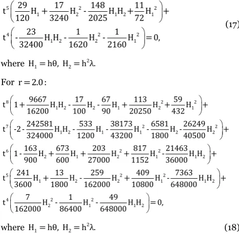
For r = 0.5:
8 2 2
1 1 2 1 2 2
7 2 2
1 2 1 2 2 1
6 2 2
1 2 1 2 1 2
5
71 3881 146 89 217
t 1+ H + H H - H - H + H +
675 81000 225 600 40500
18596 4 3317 17473 1318
t -2 - H H + H - H - H - H +
10125 25 900 20250 675
28 47 69263 271 811
t 1 - H - H - H H + H - H +
75 360 27000 225 13500
194 t H 225 2 2
1 2 1 2 2 1
4 2 2
1 2 2 1
8 7943 794 442
- H - H H + H + H +
225 20250 10125 675
4 76 8
t - H H - H - H = 0,
10125 10125 675
where 2
1 2
H = hθ, H = h λ. (16)
For r =1.0 :
8 2 2
1 2 2 1 2 1
7 2 2
1 2 2 1 2 1
6 2 2
2 1 2 1 2 1
1777 29 251 19 29
t 1+ H H - H - H + H + H +
32400 180 360 3240 240
2173 331 131 2257 1273
t -2 - H H - H - H - H - H +
2025 90 360 3240 1080
29 59 1 5863 163
t 1 - H + H - H - H H + H +
180 72 360 5400 180
13
5 2 2
1 2 1 2 1
4 2 2
1 2 2 1
29 17 148 11
t H + H - H H + H +
120 3240 2025 72
23 1 1
t - H H - H - H = 0,
32400 1620 2160
(17)
where 2
1 2
H = hθ, H = h λ.
For r = 2.0 :
8 2 2
1 2 2 1 2 1
7 2 2
1 2 1 1 2 2
6 2 2
2 1 2 1 1 2
9667 17 67 113 59
t 1+ H H - H - H + H + H +
16200 100 90 20250 432
242581 533 38173 6581 26249
t -2 - H H - H - H - H - H +
324000 1200 43200 1800 40500
163 673 203 817 21463
t 1 - H + H + H + H - H H
900 600 27000 1152 36000
5 2 2
1 2 2 1 1 2
4 2 2
2 1 1 2
+
241 13 259 409 7363
t H + H - H + H - H H +
3600 1800 162000 10800 648000
7 1 49
t H - H - H H = 0,
162000 86400 648000
where 2
1 2
H = hθ, H = h λ. (18)
The boundary of the absolute stability region in H - H1 2plane
is determined by substituting t with 1,-1 and eiθ for
0 θ 2πin the stability polynomial which is done by using MAPLE. Figure 2 illustrates the region of the absolute stability with various values of rthat lies inside the boundary traced by the dotted lines and the axes. The stability region gets bigger as the step size ratio increases. This indicates that the method provides a better accuracy with smaller step size.
Figure 2. Stability region of two-point diagonally block method
C. Implementation
This study uses shooting technique for solving the BVPs of (1) with Robin conditions. The underlying concept of shooting technique is to transfrom BVPs into initial value problems (IVPs) which requires the initial guessing to represent the missing initial condition. Our shooting strategy works as
follows. At first, we rewrite equation (1) into the following IVPs form
(
)
y = f x,y,y , x [a,b]
with couple of the initial conditions
1 1 1 1 1
y (a) = s , y (a) = V - Cy (a)
where 1
1
1 2
α c
V = , C =
c c and s1is the guessing value. Next,
we perform the computation using the proposed predictor and corrector formulas until end of the interval and verify the stopping condition given by
( )
( )
(
1 1)
g y b ,y b -β < TOL
where TOL is the tolerance that has been set while
( )
( )
(
1 1)
3( )
4( )
g y b , y b = c y b + c y b . The iteration is
repeated until we reach the prescribed stopping condition while the guessing value, sj for j = 2,3,…will be corrected
using Newton divided difference interpolation technique. In this study, the first two guessing values are chosen as
1
s = 0and s = 12 because we adopt a strategy similar to
Roberts, 1979 where both initial estimates were used to initialize the iterative solver.
In our code, the formulation to estimate the local truncation error, LTE,applied in the conditional statement
while checking for the step size selection is based on the absolute difference between the derived corrector formula of order pwith the corrector formula of order p - 1,both at
the first point. For example,
(
)
2
n-2 n-1 n n+1 h
LTE = 58f - 144f +108f - 18f 720
is used as an estimator of LTE at xn+1 for the 2PDVS
method when r =0.5. The choice of the next step size
depends on the test comparison between LTE and TOLas
follows:
• Case 1: If LTE TOL, the successful step is achieved.
The step size ratio can be chosen as either r =1.0or
r =0.5.For r = 1.0,the next step size is fixed. On the
other hand, for r = 0.5, the next step size will be
doubled.
• Case 2: If LTE > TOL, then the failure step is
14 If the integration steps are successful, then the next step size prediction is given by
1 k+1
new old TOL h =δ× h ×
LTE
(19)
(
new old)
new old new oldif h > 2× h , then h = 2× h else h = h
where δ =0.5is a safety factor while kis the order of the LTE
formula.
Algorithm of 2PDVS
Step 1 : Set TOL and calculate the initial guesses,
1 1 1 1 1
y (a) = s , y (a) = V - Cy (a).
Step 2: Calculate the initial step size.
Step 3: Compute a set of starting values using the direct Euler and modified Euler method.
Step 4: Compute the approximate values of y , y ,fp p p for
p = 3,4 using the derived predictor and corrector
formulas with m
PE(CE) where m = 1,2,… until it
converges using the convergence test at each iteration.
Step 5: Calculate the LTE and determine for the step size selection; if LTE TOL, the step is a success. Apply
the step size formula as given in (19) else halving the
step size with new old
1 h = × h .
2
Step 6: If x +2h4 new> b, then 4
final b - x
h = .
2 Go to Step 7.
Else, hnew remains as calculated. Set
i i+2 i i+2 i i+2 i i+2
x = x ,y = y ,y = y ,f = f , for i = 0,1,2.
Repeat Step 4.
Step 7: Reset the values of five back values using interpolation approach with hfinal.
Step 8: At x = b,4 verify the stopping condition.
If g y b ,y b -β
(
j( ) ( )
j)
TOL is satisfied, then go to Step 10. Else, continue Step 9.Step 9: Generate the new guessing values, y (a) = sj j and
j 1 j
y (a) = V - Cy (a) for j = 2,3,…based on the previous
guesses using the Newton divided difference interpolation formula. Repeat Step 2.
Step 10: Execute the results. Complete.
In this study, the calculation of the maximum numerical error (MAXE) in the computed block is given by
( )
( )
p p 3 p 4
p y x - y
MAXE = max .
A + By x
On the other hand, the convergence test formula is given by
(
)
n+1,m n+1,m-1
n+1,m y - y
< 0.1× TOL . A + B y
We assigned the values of A = 1and B = 1in the above two formulas which corresponds to the mixed test.
III. RESULTS AND
DISCUSSION
In this section, we consider two numerical tested problems to provide a clear view regarding the practical usefullness of the 2PDVS method. The following notation is used in the following results.
MAXE : Maximum error
h : step size
TOL : Tolerance
TS : Total step at last iteration
FS : Failure step
FCN : Total function call TG : Total iteration of guess Time : Time computation in second
2PDD4 : Direct two-point diagonal block method of order four developed in Nasir et al., (2018)
2PDVS : Direct two-point diagonally block method with variable step size proposed in this study
Problem 1. Given the following linear second order differential equation
π y = y - 2cos(x), x π
2
withy π +3y π = -1
2 2
and y
( )
π + 4y π = -4.( )
Exact solution : y(x) = cos(x).
Source: Islam and Shirin, (2011)
Problem 2. Given the following nonlinear second order differential equation
( )
(
2)
-x 2 1
y = e y + y , 0 x 1 2
with y 0 - y 0 = 0
( ) ( )
and y 1 + y 1 = 2e.( )
( )
15 All the computation results for 2PDVS are computed using C language in Code::Blocks 16.01 platform where we have compared the performances of 2PDVS with 2PDD4 method. Both method satisfies the method of order four and in the form of diagonally block multistep method features. In addition, 2PDVS and 2PDD4 were implemented using the similar shooting strategy, but the latter method used the constant step
size in its formulation
.
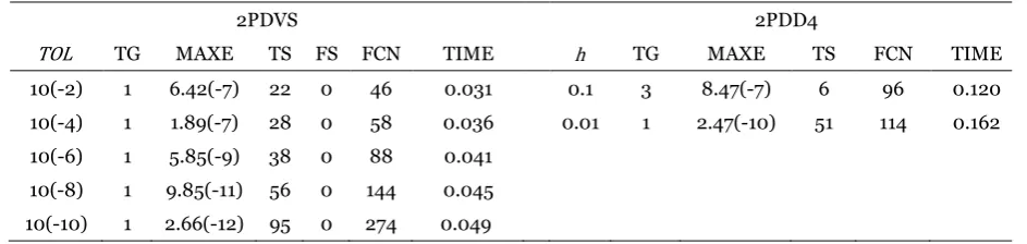
In Table 1, tabulated data shows that 2PDVS requires only single iterations at TOL10(-2)to satisfy the provided terminal
value compare to 2PDD4 that acquires three initial guesses at
h = 0.1with comparable accuracy. At the same time, the total
function calls for 2PDVS is lesser than 2PDD4. At TOL10(-8),
2PDVS achieved high accuracy results with additional five steps than 2PDD4 at h = 0.01for solving Problem 1.
2PDVS requires half number of total guesses at TOL10(-2)
compared to 2PDD4 at h = 0.1for solving Problem 2 with
comparable accuracy. As can be seen in Table 2, 2PDVS manages to achieve the same accuracy with the accuracy obtained by 2PDD4 at h = 0.01but with less steps and less
total function calls.
Overall observation from the numerical results displayed in Tables 1 - 2 show that the execution time for 2PDVS is faster than 2PDD4. This is expected since the algorithm of 2PDVS
undergo the step size selection which allowed to double from the previous step size in the succesful block.
IV. CONCLUSION
In this research, we have shown that the proposed
two-point diagonally block method is suitable for solving the
second order Robin type BVPs directly with variable step
size strategy. This method manages to preserve the
accuracy of the numerical results, economically in terms
of total steps and better in execution time when
comparing with the existing method.
V. ACKNOWLEDGEMENTS
The authors gratefully acknowledge the financial support
received from Putra Grant (Project Code:
GP-IPS/2018/9625100), Universiti Putra Malaysia (UPM)
and SLAB Scholarship sponsored by the Ministry of
Education (MOE), Malaysia. Table 1. Comparison of the numerical results for solving Problem 1
2PDVS 2PDD4
TOL TG MAXE TS FS FCN TIME h TG MAXE TS FCN TIME
10(-2) 1 6.42(-7) 22 0 46 0.031 0.1 3 8.47(-7) 6 96 0.120
10(-4) 1 1.89(-7) 28 0 58 0.036 0.01 1 2.47(-10) 51 114 0.162
10(-6) 1 5.85(-9) 38 0 88 0.041
10(-8) 1 9.85(-11) 56 0 144 0.045
10(-10) 1 2.66(-12) 95 0 274 0.049
Table 2. Comparison of the numerical results for solving Problem 2
2PDVS 2PDD4
TOL TG MAXE TS FS FCN TIME h TG MAXE TS FCN TIME
10(-2) 2 2.48(-7) 19 0 81 0.036 0.1 4 4.90(-7) 6 120 0.131
10(-4) 2 1.61(-7) 26 0 109 0.042 0.01 2 1.90(-11) 51 228 0.182
10(-6) 2 2.17(-8) 34 0 145 0.047
10(-8) 2 4.75(-11) 47 0 201 0.049
16
VI. REFERENCES
Anakira, NR, Alomari, AK, Jameel, AF, & Hashim, I 2017, ‘Multistage optimal homotopy asymptotic method for solving boundary value problems with robin boundary conditions’, Far East Journal of Mathematical Sciences, vol. 102, no. 8, pp. 1727–1744.
Awoyemi, DO, Adebile, EA, Adesanya, AO & Anake, TA 2011, ‘Modified block method for the direct solution of second order ordinary differential equations’, International Journal of Applied Mathematics and Computation, vol. 3, no. 3, pp. 181–188.
Cuomo, S. & Marasco, A. 2008, ‘A numerical approach to nonlinear two-point boundary value problems for ODEs’, Computers & Mathematics with Applications, vol. 55, no. 11, pp. 2476–2489.
Duan, JS, Rach, R, Wazwaz, AM, Chaolu, T & Wang, Z 2013, ‘A new modified Adomian decomposition method and its multistage form for solving nonlinear boundary value problems with Robin boundary conditions’, Applied Mathematical Modelling, vol. 37, no. 20–21, pp. 8687–8708.
Islam, MS & Shirin, A 2011, ‘Numerical Solutions of a Class of
Second Order Boundary Value Problems on Using Bernoulli
Polynomials’, Applied Mathematics, vol. 2, no. 9, pp. 1059–
1067.
Jator, SN 2010, ‘Solving second order initial value problems by a hybrid multistep method without predictors’, Applied Mathematics and Computation, vol. 217, no. 8, pp. 4036– 4046.
Lambert, J.D., 1973. Computational Methods in Ordinary Differential Equations, London; New York: Wiley.
Lang, FG & Xu, XP 2012, ‘Quintic B-spline collocation method
for second order mixed boundary value problem’, Computer Physics Communications, vol. 183, no. 4, pp. 913–921. Nasir, NM, Majid, ZA, Ismail, F & Bachok, N 2018, ‘Diagonal
Block Method for Solving Two-Point Boundary Value Problems with Robin Boundary Conditions’, Mathematical Problems in Engineering, 2018.
Phang, PS, Majid, ZA, Ismail, F, Othman, KI & Suleiman, M
2013, ‘New algorithm of two-point block method for solving
boundary value problem with dirichlet and Neumann
boundary conditions’, Mathematical Problems in
Engineering, 2013.
Rach, R, Duan, JS & Wazwaz, AM 2016, ‘Solution of Higher-Order, Multipoint, Nonlinear Boundary Value Problems with High-Order Robin-Type Boundary Conditions by the Adomian Decomposition Method’, Applied Mathematics & Information Sciences, vol. 10, no. 4, pp. 1231–1242.
Roberts, C.E., 1979. Ordinary differential equations: a computational approach, Englewood Cliffs, NJ: Prentice-Hall.
Waeleh, N & Majid, ZA 2017, ‘Numerical algorithm of block
method for general second order ODEs using variable
step size’, Sains Malaysiana, vol. 46, no. 5, pp. 817–
![Figure 1. visualizes the interval [a,b] divided into a series of](https://thumb-us.123doks.com/thumbv2/123dok_us/8429296.1697178/2.596.65.284.84.185/figure-visualizes-interval-b-divided-series.webp)